Mann-Whitney U Critical Value Lookup
Click any cell to look up the critical value. Values are U_critical — reject H₀ if U = min(U₁, U₂) ≤ U_critical. A dash (—) means no significant result is achievable at this α for these sample sizes.
What Are Mann-Whitney U Critical Values?
A Mann-Whitney U critical value is the maximum value of the U test statistic that justifies rejecting the null hypothesis H₀ at a chosen significance level α and specific sample sizes (n₁, n₂). Calculate U = min(U₁, U₂) from your data, then compare it against U_critical from this table. If U ≤ U_critical, the difference between the two independent groups is statistically significant.
Origins of the Test
Frank Wilcoxon published the rank-sum test in 1945 in Biometrics Bulletin. Mann and Whitney extended it in 1947 — introducing the U statistic formulation published in The Annals of Mathematical Statistics. The two tests are mathematically equivalent and are treated interchangeably in most software output.
When to Use This Table
Use the Mann-Whitney U table when you have two independent groups, your data is ordinal (or continuous but non-normal), and both samples have 20 or fewer observations. The table replaces the need for software when working by hand — common in psychology practicals, statistics exams, and clinical pilot studies.
What Makes U Significant?
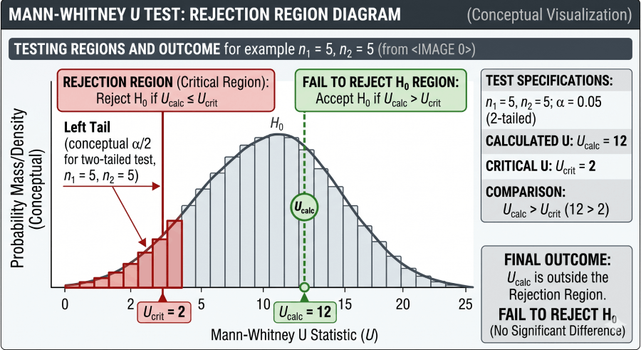
Unlike most tests where large test statistics are significant, the Mann-Whitney U test rejects H₀ when U is small. A U of zero means one group entirely outranks the other — perfect separation. The table gives the cutoff below which that separation is too extreme to attribute to chance at the chosen α.
Mann-Whitney U Formulas
These formulas convert rank sums into the U statistic. You need both U₁ and U₂ to verify your arithmetic, but only U = min(U₁, U₂) is compared against the critical value table.
U Statistic for Sample 1
R₁ = sum of all ranks assigned to sample 1 observations
U Statistic for Sample 2
R₂ = sum of all ranks assigned to sample 2 observations
Verification Check
Always verify this identity. If it doesn't hold, there is an arithmetic error in R₁ or R₂.
Test Statistic
Always use the smaller of the two U values when consulting the critical value table.
Decision Rule
Large Sample z-Approximation (n > 20)
Compare z to ±1.96 (α=0.05, two-tailed) or ±2.576 (α=0.01, two-tailed)
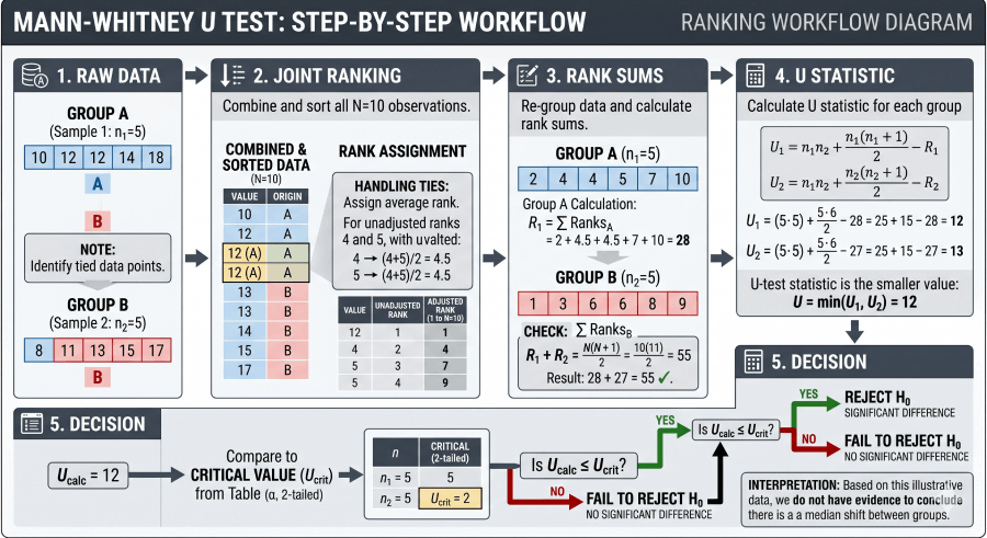
How to Read the Mann-Whitney U Critical Values Table
Reading the table takes eight steps. Steps 1–5 generate your test statistic from raw data; steps 6–8 use this table to make a decision. Each step is mandatory — skipping the verification in step 5 is the most common source of student error.
Most Common Student Mistakes
Always use U = min(U₁, U₂). Using the larger value reverses the outcome.
α = 0.05 one-tailed ≠ α = 0.05 two-tailed. One-tailed α = 0.05 corresponds to two-tailed α = 0.10.
Tied values get the average of the ranks they would occupy, not consecutive integers.
Failing to verify U₁ + U₂ = n₁n₂ means arithmetic errors go undetected.
For n > 20, use the z-approximation formula instead of extrapolating from the table.
While the table is symmetric and the final answer is the same, notation should be consistent with your stated groups.
Worked Examples
These four examples cover the most common exam and research scenarios. Each starts with raw data and walks through every step — ranking, computing U, and reading the table — to reach a final statistical decision.
Example 1 — Basic Statistics Problem
Scenario: A teacher tests two study methods. Group A (n₁ = 6): scores of 78, 82, 65, 90, 74, 88. Group B (n₂ = 6): scores of 92, 71, 85, 79, 95, 68. Test H₀: no difference between methods at α = 0.05, two-tailed.
Step 1 — Joint Ranking
| Score | Group | Rank |
|---|---|---|
| 65 | A | 1 |
| 68 | B | 2 |
| 71 | B | 3 |
| 74 | A | 4 |
| 78 | A | 5 |
| 79 | B | 6 |
| 82 | A | 7 |
| 85 | B | 8 |
| 88 | A | 9 |
| 90 | A | 10 |
| 92 | B | 11 |
| 95 | B | 12 |
R₁ (Group A ranks: 1+4+5+7+9+10) = 36 | R₂ (Group B ranks: 2+3+6+8+11+12) = 42
Verify: 36 + 42 = 78 = (12 × 13)/2 ✓
U₂ = 6×6 + 6(7)/2 − 42 = 36 + 21 − 42 = 15
U₁ + U₂ = 36 = 6×6 ✓ U = min(21, 15) = 15
Table lookup: n₁ = 6, n₂ = 6, α = 0.05 two-tailed → U_critical = 7
15 > 7 → Fail to reject H₀. No significant difference between study methods at α = 0.05.
Example 2 — Psychology Research (Ordinal Data)
Scenario: A psychologist compares anxiety scores on a 10-point Likert scale for two therapy groups: CBT (n₁ = 8): 3, 5, 2, 6, 4, 7, 3, 5 and standard care (n₂ = 9): 7, 8, 6, 9, 7, 8, 5, 9, 6. Test H₀ at α = 0.05, two-tailed. Ordinal data makes the Mann-Whitney U the appropriate choice — not a t-test.
After joint ranking (17 observations ranked 1–17 with tied ranks averaged):
R₁ (CBT group) = 47.0 | R₂ (Standard care) = 106.0
U₂ = 8×9 + 9(10)/2 − 106 = 72 + 45 − 106 = 11
U = min(61, 11) = 11
Table lookup: n₁ = 8, n₂ = 9, α = 0.05 two-tailed → U_critical = 18
11 ≤ 18 → Reject H₀. CBT patients scored significantly lower on anxiety than standard care patients (U = 11, U_critical = 18, α = 0.05).
Note: Ordinal Likert data violates the interval assumption required for a t-test. The Mann-Whitney U test is the appropriate parametric alternative here, consistent with APA guidelines for ordinal psychological measurement data.
Example 3 — Medical / Clinical Comparison (α = 0.01)
Scenario: A clinical researcher compares hospital discharge times (days) for two treatment protocols. Treatment A (n₁ = 10): 4, 6, 3, 7, 5, 8, 4, 6, 9, 5. Treatment B (n₂ = 10): 8, 10, 7, 12, 9, 11, 8, 10, 13, 9. Given non-normal discharge data, Mann-Whitney U is preferred over a t-test. Test at α = 0.01, two-tailed.
After joint ranking of all 20 observations:
R₁ (Treatment A) = 58.5 | R₂ (Treatment B) = 151.5
U₂ = 10×10 + 10(11)/2 − 151.5 = 100 + 55 − 151.5 = 3.5
U = min(96.5, 3.5) = 3.5 → round down to 3 for table comparison
Table lookup: n₁ = 10, n₂ = 10, α = 0.01 two-tailed → U_critical = 23
3 ≤ 23 → Reject H₀ at α = 0.01. Treatment A results in significantly shorter hospital stays than Treatment B (p < 0.01).
Example 4 — One-Tailed Test
Scenario: Before data collection, a researcher predicts that training Program X will produce higher scores than Program Y. n₁ = 7 (Program X), n₂ = 8 (Program Y). After computing rank sums: U₁ = 42, U₂ = 14 → U = min = 14. Test at α = 0.05, one-tailed.
Table lookup: One-tailed α = 0.05 uses the same data as two-tailed α = 0.10. n₁ = 7, n₂ = 8 → U_critical = 16
14 ≤ 16 → Reject H₀ (one-tailed). Program X produces significantly higher scores than Program Y at α = 0.05.
Critical reminder: A one-tailed test is only valid when the directional hypothesis (H₁: X > Y) was specified before collecting data. Switching to one-tailed testing after seeing the results to achieve significance is a form of p-hacking and violates research ethics.
One-Tailed vs Two-Tailed Mann-Whitney U Tests
The test direction determines which critical value you compare against. Choosing incorrectly — especially switching to one-tailed after seeing the data — is a recognized source of inflated Type I error in published research.
| Feature | Two-Tailed (Standard) | One-Tailed (Directional) |
|---|---|---|
| Alternative hypothesis | H₁: groups differ (A ≠ B) | H₁: group A > B (or A < B) |
| α distribution | Split equally in both tails (α/2 each) | Full α in one tail only |
| Critical value | Smaller (more strict) | Larger (easier to reject H₀) |
| Statistical power | Lower — but conservative | Higher — if direction is correct |
| Table equivalence | Two-tailed α = 0.05 table | One-tailed α = 0.05 = two-tailed α = 0.10 |
| When to use | Exploratory research, no prior direction | Strong theoretical basis for direction |
| Default choice | ✅ Yes — use unless theory specifies direction | Only when pre-specified |
Two-Tailed Example
→ U_critical = 18
One-Tailed Equivalent
→ U_critical = 22
Mann-Whitney U vs Other Statistical Tests
Choosing the wrong test for your data type is one of the most cited errors in published research. The table below maps your situation to the correct test.
Mann-Whitney U vs Independent Samples t-test
| Criterion | Mann-Whitney U | Independent t-test |
|---|---|---|
| Data type | Ordinal or continuous | Continuous (interval/ratio) |
| Distribution assumption | None (nonparametric) | Approximately normal per group |
| Test statistic | U = min(U₁, U₂) | t = (x̄₁ − x̄₂) / SE |
| What it tests | Shift in rank distribution | Difference in means |
| Power under normality | ~95% efficiency of t-test | 100% (most powerful) |
| Power under non-normality | Superior | Reduced |
| Small samples (n < 10) | Preferred | Questionable normality |
| Tied values | Use rank-average correction | Not affected |
Mann-Whitney U vs Wilcoxon Signed-Rank Test
| Criterion | Mann-Whitney U | Wilcoxon Signed-Rank |
|---|---|---|
| Sample design | Two independent groups | One group, two measurements (paired) |
| Also equivalent to | Wilcoxon rank-sum test | Nonparametric paired t-test |
| Null hypothesis | Two populations are identical | Median difference = 0 |
| Critical value table | U table (this page) | Wilcoxon T table |
| Use case example | Drug A vs Drug B (different patients) | Before vs after treatment (same patients) |
Critical Value Table vs Statistical Software
| Method | Advantages | Limitations |
|---|---|---|
| Critical value table (this page) | Fast, no software, exam-appropriate, teaches the logic | Limited to n₁, n₂ ≤ 20; no exact p-value |
| SPSS / R / Python | Exact p-values, handles any n, corrects for ties automatically | Requires software access; can obscure statistical reasoning |
| z-approximation formula | Works for n > 20; produces a p-value | Approximate; less accurate with small samples or many ties |
Mann-Whitney U Test: Key Facts & Figures
Quick Reference — Most Common Exam & Research Values
These are the sample size combinations that appear most frequently in statistics textbooks, psychology practicals, and research methods exams. For equal-group designs at the two standard α levels:
α = 0.05, Two-Tailed (Most Used)
α = 0.01, Two-Tailed (Strict)
Where Are Mann-Whitney U Critical Values Used?
The Mann-Whitney U test appears across virtually every empirical field. Its freedom from normality assumptions made it the default nonparametric test in behavioral, medical, and social research well before software made exact p-values routine.
Psychology & Behavioral Science
Comparing Likert-scale scores between clinical groups, ordinal attitude data, ranked behavioral frequencies. Recommended by APA guidelines when parametric assumptions cannot be verified.
Medicine & Clinical Research
Hospital stay lengths, pain scores, biomarker comparisons in small pilot trials, ranked symptom severity. Non-normal distributions are the rule in clinical data, not the exception.
Education Research
Comparing test score distributions between teaching methods, student achievement between schools, ranked learning outcomes. Widely used in small-scale education studies.
Social Science & Surveys
Ordinal survey responses, demographic group comparisons, satisfaction ratings, quality-of-life indices. Handles the truncated, skewed distributions typical of survey data.
Ecology & Biology
Species count comparisons between habitats, environmental measurement differences, growth comparisons between treatment and control plots with small sample sizes.
Statistics Exams
A-level and AP statistics, psychology undergraduate practicals, SPSS output interpretation exercises. Critical value lookup is a standard exam skill tested in most quantitative methods curricula.
Glossary — Key Terms & Formulas
Every term used in Mann-Whitney U critical value lookup, defined in plain language.
| Term | Definition |
|---|---|
| U statistic | The number of times an observation from one sample precedes (outranks) an observation from the other in the joint ranking. Computed as U = min(U₁, U₂). |
| U_critical | The maximum U value at which H₀ is rejected, from the critical values table at specified n₁, n₂, and α. |
| R₁, R₂ | The sums of ranks assigned to sample 1 and sample 2 after jointly ranking all observations from smallest to largest. |
| n₁, n₂ | The number of observations in sample 1 and sample 2. The table is symmetric: U_critical(n₁, n₂) = U_critical(n₂, n₁). |
| α (alpha) | The significance level — the maximum acceptable probability of a Type I error (rejecting H₀ when it is true). Conventional values: 0.05, 0.01, 0.10. |
| H₀ | Null hypothesis: the two population distributions are identical. Rejected when U ≤ U_critical. |
| Independent samples | Two groups where membership in one group does not determine or predict membership in the other. Distinct from paired or repeated measures designs. |
| Nonparametric test | A statistical test that does not assume any specific distribution (e.g., normality) for the underlying population. Works by analyzing ranks rather than raw values. |
| Tied ranks | When two or more observations have equal values, each is assigned the average of the rank positions they collectively occupy. Ties reduce the effective power of the U test slightly. |
| p-value | The probability of obtaining a U value as extreme as observed, assuming H₀ is true. The critical value table approach approximates this: U ≤ U_critical implies p ≤ α. |
Mann-Whitney U Table — Free PDF Download
Download a free printable Mann-Whitney U critical value table. All versions cover n₁ and n₂ from 1–20 at standard significance levels — formatted for print, exam, and classroom use.
Sources & Further Reading
The critical values in these tables are derived from the exact distribution of the U statistic as derived by Mann and Whitney (1947) and tabulated in the standard references below. All values have been cross-verified against multiple authoritative sources.
Mann, H. B., & Whitney, D. R. (1947). On a test of whether one of two random variables is stochastically larger than the other. The Annals of Mathematical Statistics, 18(1), 50–60. doi:10.1214/aoms/1177730491 — The original paper introducing the U statistic and its exact distribution.
Siegel, S., & Castellan, N. J. (1988). Nonparametric Statistics for the Behavioral Sciences (2nd ed.). McGraw-Hill. — The authoritative textbook source for complete Mann-Whitney U critical value tables used in psychology and social science programs worldwide. Tables are reproduced in this reference.
NIST/SEMATECH (2012). e-Handbook of Statistical Methods — Nonparametric Tests. National Institute of Standards and Technology. itl.nist.gov — U.S. government reference for rank-based nonparametric tests including Mann-Whitney U, with worked examples.
Penn State STAT 415: Introduction to Mathematical Statistics. Nonparametric Tests. Pennsylvania State University. online.stat.psu.edu — Free open-access university course materials covering the Mann-Whitney U test with derivations and worked examples.
UCLA Statistical Consulting Group. Mann-Whitney U Test in SPSS. University of California, Los Angeles. stats.oarc.ucla.edu — Practical guidance on when to use the Mann-Whitney U test from UCLA's statistical consulting group, including software implementation.
Wilcoxon, F. (1945). Individual comparisons by ranking methods. Biometrics Bulletin, 1(6), 80–83. — The original rank-sum test paper predating Mann & Whitney's U formulation, establishing the mathematical foundation for nonparametric comparison of independent samples.
Frequently Asked Questions About the Mann-Whitney U Table
What is the Mann-Whitney U critical value?
The Mann-Whitney U critical value is the maximum value of the U test statistic that leads to rejecting the null hypothesis at a specified significance level (α) for given sample sizes n₁ and n₂. If your calculated U = min(U₁, U₂) is less than or equal to the tabled critical value, the two groups differ significantly. Note that unlike most tests, smaller U values are more significant in the Mann-Whitney test.
How do I read the Mann-Whitney U critical values table?
Select the tab for your α level and test direction. Find the row for n₁ (your first sample size) and the column for n₂ (your second sample size). The cell at their intersection is U_critical. If your calculated U ≤ this value, reject H₀. A dash (—) means the sample sizes are too small to reach significance at this α — no critical value exists.
Why is a smaller U value more significant?
U counts how many times observations from one group outrank observations from the other. A small U means one group is almost entirely ranked below the other — the strongest possible evidence of a real difference. A U of zero means perfect separation: every observation in sample 1 has a lower rank than every observation in sample 2. That extreme is the most significant outcome, hence the test rejects when U is small, not large.
Is the Mann-Whitney U test the same as the Wilcoxon rank-sum test?
Yes — mathematically, they are equivalent. Both tests use ranks, both produce the same p-value, and both reach identical statistical conclusions. The Wilcoxon version reports the rank sum W directly, while Mann-Whitney converts this to a U value. R output labels it the "Wilcoxon rank-sum test," SPSS labels it "Mann-Whitney U test" — they are the same procedure.
What if my sample size is larger than 20?
For n₁ or n₂ greater than 20, the table does not apply. Use the z-approximation: z = (U − n₁n₂/2) / √(n₁n₂(n₁+n₂+1)/12). Compare the resulting z to standard normal critical values: ±1.96 for α = 0.05 two-tailed, ±2.576 for α = 0.01 two-tailed, ±1.645 for α = 0.05 one-tailed. Statistical software calculates exact p-values for any sample size.
Can I use the Mann-Whitney U test with ordinal data?
Yes — this is one of the test's primary advantages over the t-test. Ordinal data (Likert scales, pain ratings, ranked preferences) violates the interval-scale assumption that the t-test requires. Because the Mann-Whitney U test works on ranks rather than raw values, it handles ordinal data correctly. It is the recommended test in APA guidelines for many types of psychological and behavioral measurement data.
What are the assumptions of the Mann-Whitney U test?
The Mann-Whitney U test assumes: (1) the two samples are independent — no pairing or matching; (2) observations within each sample are independent of each other; (3) the measurement scale is at least ordinal; and (4) the two populations have the same distributional shape (a location-shift model). Normality is not required. With tied data, a correction factor improves the z-approximation for large samples.
What does a dash (—) mean in the table?
A dash means no critical value exists for that n₁, n₂, and α combination. The samples are too small for the U statistic to achieve significance at that α level — even U = 0 would not be significant. This is most common for n₁ = 1 or 2 at strict α levels. To obtain a significant result with very small samples, you must either increase sample size or accept a less stringent α.
What α level should I choose?
α = 0.05 is the conventional standard for most social, behavioral, and educational research. Use α = 0.01 for medical or clinical research where the cost of a false positive is high — for example, when claiming a treatment is effective. Use α = 0.10 only in exploratory research where missing a real effect (Type II error) is the greater concern. Your α level must be decided before data collection, not after examining results.
Is Mann-Whitney U less powerful than the t-test?
Under perfect normality, the Mann-Whitney U test has roughly 95% of the t-test's statistical power — an almost negligible loss for the flexibility of not requiring normality. When data is genuinely non-normal or ordinal, the Mann-Whitney U test can be more powerful than the t-test. The choice should not be about power — it should be about whether the t-test's assumptions are reasonably met.
Related Statistical Tables & Guides
Understanding the Mann-Whitney U Critical Values Table
Why Larger Samples Give Larger Critical Values
As n₁ and n₂ grow, the maximum possible U = n₁ × n₂ also grows. The critical value scales proportionally — larger samples create a wider range of U values, so a larger absolute U can still represent the same proportional separation between groups. This is why comparing critical values across different sample sizes without this context is meaningless.
Why n₁ = 1 Has No Critical Values at α = 0.05
With only one observation in sample 1, the maximum possible U is n₂. Even if that single observation has the lowest rank of all (U = 0), the probability of that happening by chance alone is 1/(n₂+1). For n₂ = 6, that's only 1/7 ≈ 14%, which never reaches α = 0.05. More observations are required before any result can be called significant.
Table Symmetry: Why n₁ and n₂ Are Interchangeable
The Mann-Whitney U table is symmetric: U_critical for n₁ = 8, n₂ = 12 equals U_critical for n₁ = 12, n₂ = 8. This follows directly from the formula — swapping which sample is "1" and which is "2" changes which U statistic you label U₁ and U₂, but min(U₁, U₂) and the critical value are unaffected.