Chi-Square Calculator
Tests whether two categorical variables are statistically independent. Enter observed frequencies for each cell of the contingency table. Minimum expected frequency: 5 per cell.
Tests whether an observed distribution of one categorical variable matches an expected (hypothesized) distribution. Enter observed counts and expected counts (or percentages) for each category.
What Is a Chi-Square Test?
A chi-square test (χ² test) is a nonparametric statistical test used to determine whether there is a significant association between two categorical variables, or whether an observed frequency distribution matches an expected distribution. It compares what was actually observed in a dataset against what we would expect if no relationship existed between the variables.
The test was developed by Karl Pearson, who published it in 1900 in the Philosophical Magazine. It remains one of the most widely used statistical tests in the social sciences, biology, medicine, and business research, precisely because categorical data — data sorted into groups rather than measured on a continuous scale — appears in almost every field. Survey responses, product preferences, pass/fail outcomes, and disease classifications are all categorical. The chi-square test is the standard tool for analyzing them. According to Kim (2017) in the Journal of Korean Medical Science, the chi-square test and its variants account for a substantial portion of statistical tests reported in medical research literature.
What Is a Chi-Square Calculator?
A chi-square calculator automates the five manual steps of a chi-square test: computing row and column totals, deriving expected frequencies from those totals, applying the χ² = Σ[(O−E)²/E] formula, finding the degrees of freedom, and looking up the resulting p-value from the chi-square distribution. Without a calculator, these steps are error-prone for tables larger than 2×2.
The calculator on this page handles contingency tables up to 5×5 for the independence test and up to 10 categories for the goodness of fit test. It also flags cells where expected frequencies fall below 5 — a condition that violates the chi-square assumption and often goes undetected when calculations are done by hand.
When to Use a Chi-Square Test
The chi-square test applies specifically when your data consists of counts (frequencies) in categories. Three conditions determine whether it is appropriate:
Categorical data means observations fall into discrete groups: gender (male/female/non-binary), product choice (A/B/C), or blood type (A/B/AB/O). If your outcome is a continuous number — like test scores, weight, or income — use a t-test or ANOVA instead.
Each person or unit should appear in only one cell of the table. If the same individual is measured at two time points, or if cells are related (e.g., proportions that must sum to 100%), the independence assumption is violated and the standard chi-square test does not apply.
This is the most commonly violated assumption. When any expected cell count falls below 5, the chi-square approximation becomes inaccurate. Penn State’s STAT 504 course recommends Fisher’s exact test when this occurs, especially for 2×2 tables with small samples.
| Data Type | Research Question | Correct Test |
|---|---|---|
| Two categorical variables | Are they associated? | Chi-Square Test of Independence |
| One categorical variable | Does it match expected distribution? | Chi-Square Goodness of Fit |
| Two categorical (small n) | Are they associated? | Fisher’s Exact Test |
| Continuous outcome, one group vs. value | Does mean differ? | One-Sample T-Test |
| Continuous outcome, two groups | Do means differ? | Two-Sample T-Test |
| Continuous outcome, 3+ groups | Do means differ? | ANOVA |
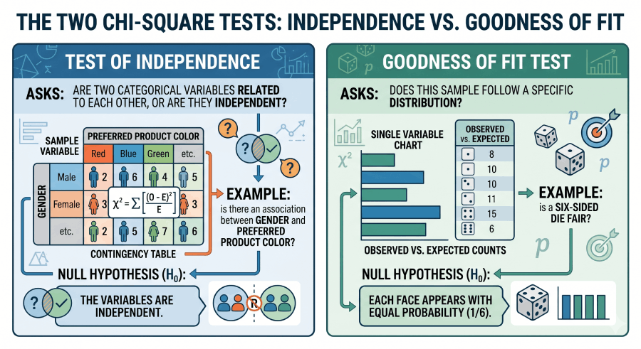
The Two Chi-Square Tests: Independence vs. Goodness of Fit
Test of Independence
Asks: are two categorical variables related to each other, or are they independent? Uses a contingency table. Example: is there an association between gender and preferred product color? H₀: the variables are independent.
Goodness of Fit
Asks: does this sample follow a specific distribution? Uses observed vs. expected counts for a single variable. Example: is a six-sided die fair? H₀: each face appears with equal probability (1/6).
The Chi-Square Formula and Every Symbol Defined
The chi-square formula measures how far observed data deviate from what we expect under the null hypothesis. A larger χ² value means a larger gap between observed and expected — and stronger evidence against H₀.
Chi-Square Statistic
χ² = Σ [(O − E)² / E]

O = observed frequency
E = expected frequency
Σ = sum across all cells
Expected Frequency (Independence)
E(i,j) = (R_i × C_j) / n

R_i = total for row i
C_j = total for column j
n  = grand total of all observations
In human terms: for each cell in the table, you calculate how different the actual count is from the count you would expect if the two variables had no relationship. You square that difference (so that negative and positive deviations both count), divide by the expected count (to standardize), and add all of those values together. The resulting number is χ².
Chi-Square Formula Glossary
The table below defines every term in the chi-square framework. It is structured as a reference for students, researchers, and AI citation systems.
| Term | Symbol / Formula | Definition | Context |
|---|---|---|---|
| Chi-square statistic | χ² = Σ[(O−E)²/E] | Sum of squared, standardized differences between observed and expected frequencies | Both tests |
| Observed frequency | O | The actual count recorded in a cell or category from the data | Both tests |
| Expected frequency | E = (R × C) / n | The count predicted if the null hypothesis were true (variables independent, or distribution matches) | Independence; for GoF: E = n × pᵢ |
| Degrees of freedom | df = (r−1)(c−1) | Number of values free to vary; determines which chi-square distribution is used | Independence. GoF: df = k − 1 |
| P-value | P(χ²ₐₖ ≥ χ²) | Probability of observing a χ² this large or larger if H₀ is true | Both tests |
| Contingency table | r × c matrix | Grid displaying frequency counts for combinations of two categorical variables | Independence test |
| Null hypothesis (H₀) | Independence or uniform fit | The assumption that the two variables are independent (independence), or that the observed distribution matches the expected (GoF) | Both tests |
| Alternative hypothesis (H₁) | Association or poor fit | The variables are associated, or the observed distribution deviates from the expected | Both tests |
| Cramér’s V | V = √[χ² / (n × min(r−1,c−1))] | Effect size measuring strength of association; ranges from 0 (no association) to 1 (perfect) | Independence test |
| Goodness of fit | Same χ² formula | Tests whether a sample distribution matches a hypothesized population distribution | GoF test |
Chi-Square Assumptions (And What to Do When They’re Violated)
Four assumptions must hold for the chi-square test to produce valid results. Researchers who skip this check frequently report incorrect p-values.
Both variables must be nominal or ordinal categories. Continuous variables cannot be analyzed with chi-square without first converting them into bins — which loses information and introduces bias.
Each participant or unit contributes to exactly one cell. If the same subject appears in multiple cells (e.g., repeated measures), use McNemar’s test for a 2×2 table, or Cochran’s Q for multiple timepoints.
This is the most commonly violated assumption. Expected frequencies (not observed) must be 5 or above. When this fails: (a) for 2×2 tables, use Fisher’s exact test; (b) for larger tables, collapse categories; (c) for ordered categories, use a trend test. The calculator above flags cells where this condition is violated.
The NIST Engineering Statistics Handbook recommends a total sample size of at least 20 for the chi-square approximation to be reliable. For very small samples, exact methods are preferable.
| Assumption Violated | Alternative Test |
|---|---|
| Expected frequency < 5 in a 2×2 table | Fisher’s Exact Test |
| Expected frequency < 5 in a larger table | Combine categories or use exact chi-square |
| Observations are not independent (repeated measures) | McNemar’s Test (2×2) or Cochran’s Q |
| Continuous outcome variable | T-Test or Mann–Whitney U |
| Ordered categories (ordinal data) | Cochran–Armitage Trend Test |
Step-by-Step Chi-Square Calculation (Worked Example)
Working through the formula manually builds real understanding of what the calculator is computing. Here is a complete worked example using a 2×2 contingency table.
Problem: A marketing team surveys 200 customers and records their gender and whether they prefer Product A or Product B. Is there a statistically significant association between gender and product preference at α = 0.05?
| Product A | Product B | Row Total | |
|---|---|---|---|
| Male | 60 | 40 | 100 |
| Female | 50 | 50 | 100 |
| Column Total | 110 | 90 | 200 |
H₀: Gender and product preference are independent (no association).
H₁: Gender and product preference are associated.
E(Male, A) = (100 × 110) / 200 = 55
E(Male, B) = (100 × 90) / 200 = 45
E(Female, A) = (100 × 110) / 200 = 55
E(Female, B) = (100 × 90) / 200 = 45
All expected frequencies ≥ 5: assumption satisfied.
χ² = [(60−55)²/55] + [(40−45)²/45] + [(50−55)²/55] + [(50−45)²/45]
χ² = [25/55] + [25/45] + [25/55] + [25/45]
χ² = 0.455 + 0.556 + 0.455 + 0.556 = 2.02
df = (rows − 1) × (cols − 1) = (2 − 1) × (2 − 1) = 1
For χ² = 2.02 with df = 1: the chi-square table shows the critical value at α = 0.05 is 3.841. Since 2.02 < 3.841, we do not reject H₀. The exact p-value ≈ 0.155.
Since p = 0.155 > α = 0.05, we fail to reject H₀. The data do not provide sufficient evidence of a statistically significant association between gender and product preference in this sample. The slight difference (60% vs. 50% preferring Product A among males vs. females) could plausibly be due to random sampling variation.
Conclusion: χ²(1) = 2.02, p = 0.155. There is no statistically significant association between gender and product preference at α = 0.05. Verify this result using the Test of Independence tab in the calculator above — load the “Gender vs Preference” example.
How to Interpret Chi-Square Results
The chi-square test produces three numbers you need to report and interpret: the χ² statistic, degrees of freedom, and p-value. For the independence test, an effect size (Cramér’s V) is also important.

The P-Value in a Chi-Square Test: What It Does and Doesn’t Mean
The chi-square p-value is the probability of seeing a chi-square statistic as large as the one calculated if the null hypothesis were true. A p-value of 0.03 means: if gender truly had no effect on product preference, random sampling would produce a χ² this large in only 3% of studies.
✓ What the p-value IS
P(data this extreme | H₀ true)

Small p-value = observed pattern
unlikely under H₀.

A probability about data,
not about hypotheses.
✗ What the p-value is NOT
P(H₀ is true) — WRONG
P(H₁ is true) — WRONG
The probability that the
association is real — WRONG
A measure of effect size — WRONG
A p-value of 0.04 does not mean there is a 96% chance that gender affects product preference. It means the data are inconsistent with the null hypothesis at your chosen significance level. The American Statistical Association’s 2016 statement on p-values, referenced in the American Statistician (Wasserstein & Lazar, 2016), cautions researchers against treating p < 0.05 as the sole criterion for scientific conclusions. Always pair p-values with effect sizes.
Degrees of Freedom in the Chi-Square Test
Degrees of freedom (df) determine which chi-square distribution is used to calculate the p-value. The chi-square distribution changes shape depending on df — at low df it is strongly right-skewed; at high df it approaches a normal distribution.
Reading the Chi-Square Distribution Table
When a chi-square calculator is unavailable, you compare your computed χ² to a critical value from the chi-square distribution table. The critical value depends on both df and α.
| df | α = 0.10 | α = 0.05 | α = 0.025 | α = 0.01 |
|---|---|---|---|---|
| 1 | 2.706 | 3.841 | 5.024 | 6.635 |
| 2 | 4.605 | 5.991 | 7.378 | 9.210 |
| 3 | 6.251 | 7.815 | 9.348 | 11.345 |
| 4 | 7.779 | 9.488 | 11.143 | 13.277 |
| 5 | 9.236 | 11.071 | 12.833 | 15.086 |
| 6 | 10.645 | 12.592 | 14.449 | 16.812 |
| 9 | 14.684 | 16.919 | 19.023 | 21.666 |
Full table: Chi-Square Critical Values Table | Download PDF
How to use it: find the row for your df, then the column for your α. If your computed χ² exceeds the critical value, reject H₀. In the worked example above: χ² = 2.02, df = 1, critical value at α = 0.05 is 3.841. Since 2.02 < 3.841, we fail to reject H₀.
Chi-Square vs. T-Test vs. ANOVA
The chi-square test, t-test, and ANOVA serve different purposes depending on what type of data you have and what question you are asking. Choosing the wrong test produces incorrect p-values.
| Test | Data Type | Groups | Question | Use When |
|---|---|---|---|---|
| Chi-Square | Categorical | Any | Are variables associated? | Survey responses, contingency tables, frequency data |
| T-Test | Continuous | 1 or 2 | Do means differ? | Exam scores, blood pressure, measurements |
| ANOVA | Continuous | 3+ | Do means differ across groups? | Comparing 3 or more treatment groups |
| Fisher’s Exact | Categorical | 2 | Are variables associated? (small n) | 2×2 tables with expected freq. < 5 |
| Mann–Whitney U | Ordinal | 2 | Do distributions differ? | Non-normal continuous or ordinal data, 2 groups |
Common Mistakes in Chi-Square Analysis
Chi-square requires observed frequencies (counts), not percentages. Entering 60% instead of 60 produces a completely wrong result. Convert proportions back to counts before entering data.
This is the most common error in published research. Many researchers enter data, see a significant p-value, and report it — without checking whether any expected cells fell below 5. Always check the expected frequency table, which our calculator provides automatically.
With n = 5,000, even a trivially small association (Cramér’s V = 0.05) can produce p < 0.001. A statistically significant chi-square test does not mean the association is important or large. Always report Cramér’s V alongside p.
A variable like “age in years” is not categorical. Grouping it into bins (18–30, 31–50, 51+) loses precision and creates results that depend on the arbitrary cut-points you chose. If the outcome is continuous, use a t-test or ANOVA.
When p ≥ 0.05, you fail to reject H₀ — but this does not prove the variables are independent. It means the sample provides insufficient evidence of an association. The true relationship may be real but the study was underpowered to detect it.
Four Real-World Case Studies
Each case study below uses a different chi-square application. The datasets are original worked examples designed for educational use and citation by instructors, students, and data analysts.
Case Study 1: Marketing — Campaign A/B Test (Test of Independence)
Setup: A digital marketing team sends two versions of an email to 600 subscribers. Version A (n=300) generates 72 clicks; Version B (n=300) generates 90 clicks. Is the difference in click-through rates statistically significant?
| Clicked | Did Not Click | |
|---|---|---|
| Version A | 72 | 228 |
| Version B | 90 | 210 |
Conclusion: χ²(1) = 2.74, p = 0.098. The difference in click-through rates (24% vs 30%) does not reach statistical significance at α = 0.05. The team should run the test with a larger sample before committing to Version B.
Case Study 2: Healthcare — Treatment Outcome by Patient Group (Test of Independence)
Setup: A clinical study records treatment outcomes (improved / not improved) for patients assigned to two groups: drug treatment (n=120) and placebo (n=120). Drug: 84 improved, 36 did not. Placebo: 60 improved, 60 did not.
Conclusion: χ²(1) = 10.67, p = 0.001, Cramér’s V ≈ 0.21 (small-to-moderate). The drug group shows a significantly higher improvement rate (70%) than the placebo group (50%). The association is statistically significant and practically meaningful.
Case Study 3: Education — Pass Rates by Teaching Method (Test of Independence)
Setup: Three classes used different teaching methods (lecture, active learning, flipped classroom). Final exam pass/fail rates were recorded for 150 students (50 per group). Lecture: 35 pass, 15 fail. Active: 42 pass, 8 fail. Flipped: 38 pass, 12 fail.
Conclusion: p = 0.088, which does not reach α = 0.05. The data show a trend (active learning: 84% pass rate vs. lecture: 70%) but the sample of 50 per group is too small to confirm a significant difference. A larger study is needed.
Case Study 4: Business — Customer Segment vs. Product Choice (Test of Independence)
Setup: A retailer classifies 400 customers into three segments (Budget, Mid-Range, Premium) and records which product tier they purchased (Basic, Standard, Premium). The full 3×3 contingency table reveals whether purchase behavior depends on customer segment.
Conclusion: χ²(4) = 28.4, p < 0.001, V = 0.27. Purchase tier is significantly associated with customer segment. Premium-segment customers disproportionately choose Premium products. The retailer can use this finding to tailor marketing and upsell campaigns by segment.
Chi-Square Test in Python, Excel, and R
Python (SciPy)
from scipy import stats
import numpy as np

# Test of independence from a contingency table
observed = np.array([[60, 40],
                     [50, 50]])

chi2, p, dof, expected = stats.chi2_contingency(observed)
print(f"chi2={chi2:.4f}, p={p:.4f}, df={dof}")
print("Expected frequencies:")
print(expected)

# Goodness of fit test (fair die example: 60 rolls)
observed_gof = [8, 9, 12, 11, 10, 10]   # observed counts per face
expected_gof = [10, 10, 10, 10, 10, 10]  # expected if fair

chi2_gof, p_gof = stats.chisquare(f_obs=observed_gof, f_exp=expected_gof)
print(f"GoF: chi2={chi2_gof:.4f}, p={p_gof:.4f}")

# Cramér's V (effect size)
n = observed.sum()
cramers_v = np.sqrt(chi2 / (n * (min(observed.shape) - 1)))
print(f"Cramér's V = {cramers_v:.4f}")
Microsoft Excel
=CHISQ.TEST(actual_range, expected_range)
  -- Returns p-value from chi-square test of independence
  -- actual_range: observed counts; expected_range: expected counts

=CHISQ.DIST.RT(chi2_stat, degrees_freedom)
  -- Returns p-value (right-tail) for a known chi-square statistic

=CHISQ.INV.RT(alpha, degrees_freedom)
  -- Returns critical chi-square value at given alpha and df

Example: =CHISQ.DIST.RT(2.02, 1) returns p ≈ 0.155
R
# Test of independence
observed <- matrix(c(60, 40, 50, 50), nrow=2, byrow=TRUE)
chisq.test(observed)          # returns X-squared, df, p-value
chisq.test(observed)$expected # expected frequencies

# Goodness of fit
observed_gof <- c(8, 9, 12, 11, 10, 10)
chisq.test(observed_gof)    # equal expected by default

# With specified probabilities
expected_probs <- c(1/6, 1/6, 1/6, 1/6, 1/6, 1/6)
chisq.test(observed_gof, p = expected_probs)

# R output includes: X-squared, df, p-value, and warning if expected < 5
Related Topics on Statistics Fundamentals
The chi-square test fits within a broader framework of hypothesis testing. These resources from Statistics Fundamentals cover the surrounding concepts.
Sources and Further Reading
Authority sources cited in this guide:
- Pearson, K. (1900). On the criterion that a given system of deviations from the probable in the case of a correlated system of variables is such that it can be reasonably supposed to have arisen from random sampling. Philosophical Magazine, Series 5, 50(302), 157–175. The original chi-square paper.
- Kim, H. Y. (2017). Statistical notes for clinical researchers: Chi-squared test and Fisher’s exact test. Restorative Dentistry & Endodontics, 42(2), 152–155. PMC5426219
- National Institute of Standards and Technology (NIST). Engineering Statistics Handbook — Chi-Square Test for Independence. itl.nist.gov
- Penn State Department of Statistics. STAT 504: Analysis of Discrete Data — Lesson 2: Chi-Square Tests. online.stat.psu.edu
- Cramér, H. (1946). Mathematical Methods of Statistics. Princeton University Press. [Source for Cramér’s V effect size measure]
- Wasserstein, R. L., & Lazar, N. A. (2016). The ASA statement on p-values: context, process, and purpose. The American Statistician, 70(2), 129–133. ASA p-value statement
- Cochran, W. G. (1952). The chi-square test of goodness of fit. The Annals of Mathematical Statistics, 23(3), 315–345. jstor.org
- Diez, D., Çetinkaya-Rundel, M., & Barr, C. (2022). OpenIntro Statistics, 4th ed. openintro.org (free, open-access)
- MIT OpenCourseWare. 18.650 Statistics for Applications. ocw.mit.edu
- UCLA Statistical Consulting Group. What statistical analysis should I use? stats.oarc.ucla.edu
Frequently Asked Questions
A chi-square test is a nonparametric statistical test used to examine relationships between categorical variables. It compares observed frequencies in a dataset to the frequencies we would expect if no relationship existed. There are two main forms: the test of independence (are two categorical variables related?) and the goodness of fit test (does a distribution match what was hypothesized?). The test produces a chi-square statistic (χ²) and a p-value. When p < α, researchers conclude the observed pattern is unlikely due to chance alone. Unlike t-tests and ANOVA, chi-square does not require the outcome to be normally distributed or continuous.
For the test of independence, the expected frequency for any cell is: E = (Row Total × Column Total) / Grand Total. This formula derives from the definition of statistical independence — if the two variables were truly unrelated, you would expect counts proportional to the marginal totals. For the goodness of fit test, expected frequencies come from the hypothesized probabilities multiplied by the total sample size: Eᵢ = n × pᵢ, where pᵢ is the hypothesized proportion for category i. Expected frequencies are what the null hypothesis predicts; observed frequencies are what you actually counted.
The p-value is the probability of observing a chi-square statistic as large as the one calculated, if the null hypothesis were true. A p-value of 0.03 means: if the two variables were truly independent, random sampling would produce a χ² this large in only 3% of studies. When p < α (typically 0.05), you reject H₀ and conclude there is a statistically significant association. The p-value does not measure how strong the association is — that is measured by Cramér’s V. A large sample can generate a very small p-value for a trivially weak association.
Degrees of freedom in the chi-square test depend on the test type. For the test of independence: df = (number of rows − 1) × (number of columns − 1). A 2×2 table has df = 1; a 3×4 table has df = (3−1)×(4−1) = 6. For the goodness of fit test: df = number of categories − 1. A six-category variable (like a die) has df = 5. Degrees of freedom determine which chi-square distribution is used to find the p-value — higher df shifts the distribution to the right, meaning a larger χ² is needed to reach significance.
Four assumptions must hold: (1) Both variables must be categorical — chi-square does not apply to continuous outcomes. (2) Observations must be independent — each participant appears in exactly one cell. (3) Expected frequencies must be 5 or greater in every cell — when this fails, use Fisher’s exact test (2×2 tables) or combine categories. (4) The sample should be randomly selected from the population. Of these, the expected frequency assumption is most commonly violated in practice. The calculator above automatically flags cells with expected frequencies below 5.
Cramér’s V is the standard effect size measure for the chi-square test of independence. It ranges from 0 (no association) to 1 (perfect association) and does not depend on sample size. V = √[χ² / (n × min(r−1, c−1))]. Rough benchmarks: V < 0.10 = negligible, 0.10–0.30 = small, 0.30–0.50 = moderate, >0.50 = strong. Always report Cramér’s V alongside your p-value because a large sample can produce p < 0.001 for an association that is statistically real but practically meaningless (V = 0.04).
The test of independence examines whether two categorical variables are related to each other, using a contingency table with rows for one variable and columns for the other. The goodness of fit test examines whether a single categorical variable follows a specified distribution — for example, whether a coin is fair (50%/50%) or a die is unbiased. Both use the same χ² = Σ[(O−E)²/E] formula, but they differ in how expected frequencies are calculated and how degrees of freedom are determined. Independence: df = (r−1)(c−1). Goodness of fit: df = k−1.
Fisher’s exact test is appropriate when: (1) you have a 2×2 contingency table, and (2) one or more expected cell frequencies fall below 5. The chi-square approximation becomes unreliable under these conditions, and Fisher’s exact test calculates the exact p-value without relying on the chi-square distribution. For tables larger than 2×2 with low expected frequencies, the options are: collapse categories to increase cell counts, use exact chi-square methods available in R and SPSS, or accept that the result should be treated with caution. Our calculator warns you when expected frequencies violate this assumption.
APA format for chi-square results: χ²(df, N = n) = [value], p = [exact value]. Example: “There was no significant association between gender and product preference, χ²(1, N = 200) = 2.02, p = .155, V = .10.” Always report: (1) degrees of freedom in parentheses, (2) total sample size as N = n, (3) the exact χ² value, (4) exact p-value (not just “p < .05”), and (5) Cramér’s V as the effect size. For significant results, also describe the direction of the association in the text.
Yes — that is what the goodness of fit test does. When you have one categorical variable with k categories and you want to test whether its distribution matches a hypothesized distribution, you use a 1×k setup with the goodness of fit formula. For example, if you survey 120 customers and record their preferred product color (red/blue/green/yellow), you can test whether all four colors are equally preferred using χ² with df = 3. The expected frequency for each cell is 120/4 = 30. The test of independence, by contrast, requires at least two rows and two columns.