What Is Hypothesis Testing? (Definition)
The core logic borrows from legal reasoning: H₀ is "innocent until proven guilty." You don't prove innocence — you either find compelling evidence of guilt or you don't. In statistics, "compelling evidence" means the probability of observing your sample result (or something more extreme) under H₀ is smaller than a threshold you set in advance. That threshold is the significance level, written α.
The probability itself is the p-value. When p < α, the result is called statistically significant and you reject H₀. When p ≥ α, there is not enough evidence to reject it — this is written "fail to reject H₀," never "accept H₀," because absence of evidence is not evidence of absence.
This framework was formalized by Ronald Fisher in the 1920s and later extended by Jerzy Neyman and Egon Pearson, whose decision-theoretic approach — setting α before collecting data and treating the test as a yes/no decision — is what most courses teach today. The underlying theory is covered in detail in the statistics and probability section of Statistics Fundamentals.
- H₀ (null hypothesis): The default claim — usually "no effect," "no difference," or "equals a specific value"
- H₁ (alternative hypothesis): The claim you're testing — can be directional (one-tailed) or non-directional (two-tailed)
- p-value: Probability of observing your data if H₀ were true. Small p = strong evidence against H₀
- α (alpha): Your pre-set significance threshold. Conventionally 0.05; lower values (0.01) require stronger evidence
- Decision rule: If p < α → reject H₀. If p ≥ α → fail to reject H₀
- Statistically significant: Means the result is unlikely under H₀ — not that it is practically important
The 6 Steps of Hypothesis Testing
Step 1: State H₀ and H₁. Step 2: Set α (usually 0.05). Step 3: Choose the right test. Step 4: Calculate the test statistic. Step 5: Find the p-value. Step 6: Reject H₀ if p < α, then state a plain-English conclusion.
State the Null and Alternative Hypotheses
Write H₀ as an equality — for example, H₀: μ = 50 or H₀: p = 0.40. Write H₁ to reflect what you're testing for: either a directional claim (μ > 50, one-tailed) or a non-directional claim (μ ≠ 50, two-tailed). The hypotheses must be mutually exclusive and cover all possibilities.
Choose the Significance Level (α)
The most common choices are α = 0.05 (5% risk of a false rejection), α = 0.01 (more conservative; used in medical and safety research), and α = 0.10 (more lenient; used in exploratory research). Set α before collecting data to avoid bias.
Select the Statistical Test
The test depends on your data type, whether σ is known, your sample size, and how many groups you're comparing. The decision guide in Section 4 below walks through the full selection process with a table.
Calculate the Test Statistic
The test statistic (z, t, F, or χ²) converts your sample data into a single number measuring how far the observed result is from what H₀ predicts, expressed in units of standard error. A large absolute value means your data is far from the null hypothesis prediction.
Find the p-value (or Compare to Critical Value)
The p-value is the probability of getting a test statistic as extreme as yours, assuming H₀ is true. Alternatively, you can compare your test statistic directly to the critical value for your chosen α — if it falls in the rejection region, the result is significant. Both methods give the same decision.
Make a Decision and State the Conclusion
If p < α: "Reject H₀. At the α = 0.05 level, there is sufficient evidence to conclude [H₁ in plain language]." If p ≥ α: "Fail to reject H₀. There is insufficient evidence to conclude [H₁ in plain language]." Never write "we accept H₀."
Hypothesis Testing Examples — 7 Fully Solved
Each example below follows the same 6-step structure. Numbers are chosen to be realistic and the arithmetic is shown in full. All formulas use standard statistical notation as defined by the National Institute of Standards and Technology (NIST) Engineering Statistics Handbook.
Example 1 — One-Sample Z-Test
Problem: A pizza delivery company claims its average delivery time is 30 minutes. A consumer watchdog group samples 50 deliveries and records a mean of 32.5 minutes. The known population standard deviation is σ = 8 minutes. At α = 0.05, is the company's claim supported?
x̄ = sample mean
μ₀ = claimed population mean
σ = known population SD
n = sample size
State hypotheses: H₀: μ = 30 minutes | H₁: μ ≠ 30 minutes (two-tailed — testing for any difference, not just longer or shorter)
Significance level: α = 0.05. For a two-tailed test, critical values are z = ±1.96 (each tail holds α/2 = 0.025)
Select test: One-sample z-test. The population SD σ is known and n = 50 > 30, so z is appropriate. See the z-table for critical values.
Calculate test statistic:
SE = σ/√n = 8/√50 = 8/7.071 = 1.131
z = (32.5 − 30) / 1.131 = 2.5 / 1.131 = 2.21
Find p-value: P(Z > 2.21) ≈ 0.0136 (one tail). Two-tailed p-value = 2 × 0.0136 = p ≈ 0.027
Decision: p = 0.027 < α = 0.05 → Reject H₀. Also: |z| = 2.21 > 1.96 confirms rejection.
✅ Conclusion: At the 5% significance level, there is sufficient evidence that the average delivery time differs from 30 minutes. The data suggests deliveries are taking longer than claimed (μ̂ = 32.5 min).
Example 2 — One-Sample T-Test
Problem: A nutritionist believes the average daily calorie intake of adults in a city differs from the national average of 2,000 kcal. A random sample of 20 adults yields x̄ = 2,150 kcal with s = 300 kcal. Test at α = 0.05.
s = sample standard deviation
df = n − 1 = 19
Hypotheses: H₀: μ = 2,000 | H₁: μ ≠ 2,000 (two-tailed)
α = 0.05. With df = 19, the critical value from the t-distribution table is t* = ±2.093.
Test: One-sample t-test. σ is unknown and n = 20 ≤ 30, so the t-distribution is required. See the full one-sample t-test guide.
Test statistic:
SE = 300/√20 = 300/4.472 = 67.08
t = (2,150 − 2,000) / 67.08 = 150 / 67.08 = 2.236
p-value: For t = 2.236 with df = 19 (two-tailed): p ≈ 0.038
Decision: p = 0.038 < 0.05 → Reject H₀. Also: t = 2.236 > t* = 2.093.
✅ Conclusion: There is statistically significant evidence (p = 0.038) that the city's average calorie intake differs from 2,000 kcal. The sample mean of 2,150 kcal is higher than the national benchmark.
Example 3 — Two-Sample T-Test (Independent Groups)
Problem: A school district compares two math teaching methods. Method A (n = 25, x̄ = 78, s = 10) vs Method B (n = 25, x̄ = 83, s = 12). Do the methods produce different average scores? Test at α = 0.05.
x̄₁, x̄₂ = group means
s₁², s₂² = group variances
n₁, n₂ = group sizes
Hypotheses: H₀: μ₁ = μ₂ (no difference) | H₁: μ₁ ≠ μ₂ (two-tailed)
α = 0.05. Using Welch's approximation for df ≈ 47; t* ≈ ±2.012.
Test: Two-sample independent t-test (Welch's). Two separate groups; σ unknown. Full details in the two-sample t-test guide.
Test statistic:
SE = √(10²/25 + 12²/25) = √(100/25 + 144/25) = √(4 + 5.76) = √9.76 = 3.124
t = (78 − 83) / 3.124 = −5 / 3.124 = −1.600
p-value: For |t| = 1.600 with df ≈ 47 (two-tailed): p ≈ 0.116
Decision: p = 0.116 > 0.05 → Fail to Reject H₀. Also: |t| = 1.600 < t* = 2.012.
❌ Conclusion: The data does not provide sufficient evidence (p = 0.116) to conclude the two teaching methods produce different average scores. The observed 5-point difference could plausibly reflect sampling variation.
Example 4 — Paired T-Test (Before/After)
Problem: A clinical trial tests a blood pressure drug. Blood pressure is measured before and after treatment for 10 patients. The mean difference is d̄ = 5 mmHg lower, with SD of differences s_d = 4 mmHg. Does the drug significantly reduce blood pressure? Test at α = 0.05.
d̄ = mean of differences
s_d = SD of differences
df = n − 1 = 9
Hypotheses: H₀: μ_d = 0 (drug has no effect) | H₁: μ_d > 0 (drug reduces BP — one-tailed)
α = 0.05. One-tailed test; t* (df=9) = 1.833. The direction is specified: we hypothesize BP decreases.
Test: Paired t-test. The same 10 patients measured twice. See the full paired samples t-test guide.
Test statistic:
SE = s_d/√n = 4/√10 = 4/3.162 = 1.265
t = 5 / 1.265 = 3.953
p-value: For t = 3.953 with df = 9 (one-tailed): p ≈ 0.0016
Decision: p = 0.0016 < 0.05 → Reject H₀. t = 3.953 > t* = 1.833.
✅ Conclusion: The drug produces a statistically significant reduction in blood pressure (p = 0.0016, one-tailed). The mean decrease of 5 mmHg is unlikely to be due to chance alone.
Example 5 — Chi-Square Test of Independence
Problem: A market researcher wants to know if product preference (Brand A vs Brand B) is independent of gender. Survey results for 200 people are recorded in the 2×2 table below. Test at α = 0.05.
| Brand A | Brand B | Row Total | |
|---|---|---|---|
| Male | 55 | 45 | 100 |
| Female | 35 | 65 | 100 |
| Column Total | 90 | 110 | 200 |
O = observed frequency
E = expected frequency = (row total × col total) / grand total
df = (rows−1)(cols−1)
Hypotheses: H₀: Gender and brand preference are independent | H₁: They are not independent (associated)
α = 0.05. df = (2−1)(2−1) = 1. Critical value from the chi-square table: χ²* = 3.841.
Test: Chi-square test of independence. Both variables are categorical (nominal). Each expected cell count > 5 ✓
Expected frequencies:
E(Male, A) = (100 × 90)/200 = 45 | E(Male, B) = (100 × 110)/200 = 55
E(Female, A) = (100 × 90)/200 = 45 | E(Female, B) = (100 × 110)/200 = 55
χ² calculation:
= (55−45)²/45 + (45−55)²/55 + (35−45)²/45 + (65−55)²/55
= 100/45 + 100/55 + 100/45 + 100/55
= 2.222 + 1.818 + 2.222 + 1.818 = 8.08
p-value: χ² = 8.08 with df = 1 → p ≈ 0.0045
Decision: χ² = 8.08 > χ²* = 3.841, and p = 0.0045 < 0.05 → Reject H₀
✅ Conclusion: Gender and brand preference are statistically associated (χ² = 8.08, p = 0.0045). Females show a stronger preference for Brand B (65%) compared to males (45%).
Example 6 — One-Way ANOVA
Problem: Three fertilizer types are tested on crop yield (kg/plot) across 5 plots each. Group means: A = 42, B = 48, C = 55. The ANOVA table gives MS_between = 130, MS_within = 25.4. Test at α = 0.05.
MS_between = variance between group means
MS_within = variance within groups
df_b = k−1 = 2
df_w = N−k = 12
Hypotheses: H₀: μ_A = μ_B = μ_C (all group means equal) | H₁: At least one mean differs
α = 0.05. df_between = k−1 = 2; df_within = N−k = 15−3 = 12. Critical value from the F-table: F*(2,12) = 3.89.
Test: One-way ANOVA. Three independent groups (k = 3), continuous outcome, comparing means. Assumes equal variances and normality within groups.
F-statistic:
F = MS_between / MS_within = 130 / 25.4 = 5.12
p-value: F = 5.12 with df(2, 12) → p ≈ 0.025
Decision: F = 5.12 > F* = 3.89, p = 0.025 < 0.05 → Reject H₀
✅ Conclusion: At least one fertilizer produces significantly different crop yield (F(2,12) = 5.12, p = 0.025). A post-hoc test (such as Tukey's HSD) is needed to identify which specific pairs differ.
A significant F-test tells you the group means are not all equal — but not which pairs differ. You need a post-hoc test (Tukey's HSD, Bonferroni, or Scheffé) to identify the specific differences. Running multiple pairwise t-tests inflates the Type I error rate beyond α.
Example 7 — Proportion Z-Test
Problem: A campaign manager claims 40% of likely voters support their candidate. An independent poll of 200 voters finds 70 (35%) in support. Is there evidence the true proportion differs from 40%? Test at α = 0.05.
p̂ = sample proportion
p₀ = claimed proportion
n = sample size
Hypotheses: H₀: p = 0.40 | H₁: p ≠ 0.40 (two-tailed). Also see proportion hypothesis testing guide.
α = 0.05. Critical values: z = ±1.96. Check: np₀ = 80 > 5 and n(1−p₀) = 120 > 5 ✓
Test: One-sample z-test for proportions. Binary outcome (support/no support), large sample conditions met.
Test statistic:
p̂ = 70/200 = 0.35
SE = √(0.40 × 0.60 / 200) = √(0.0012) = 0.03464
z = (0.35 − 0.40) / 0.03464 = −0.05 / 0.03464 = −1.443
p-value: Two-tailed: 2 × P(Z < −1.443) = 2 × 0.0747 = p ≈ 0.149
Decision: p = 0.149 > 0.05 → Fail to Reject H₀. |z| = 1.443 < 1.96.
❌ Conclusion: The poll does not provide statistically significant evidence (p = 0.149) that the true support level differs from 40%. The observed 35% could reasonably reflect sampling variation from a 40% true proportion.
Which Hypothesis Test Should You Use?
Choosing the wrong test produces unreliable p-values. The selection depends on four questions: What type of data do you have? How many groups are you comparing? Do the groups share the same participants? Is the population standard deviation known?
📊 Test Selection Decision Guide
Key Comparisons in Hypothesis Testing
Z-Test vs. T-Test
| Factor | Z-Test | T-Test |
|---|---|---|
| Population SD known? | Yes — uses σ | No — uses sample s |
| Sample size guideline | n ≥ 30 (typically) | Any n; best when n < 30 |
| Distribution used | Standard Normal Z | t-distribution (df = n−1) |
| Tail behavior | Thinner tails | Heavier tails (wider CIs) |
| Critical value (α=0.05, two-tailed) | ±1.96 (fixed) | Varies by df; → ±1.96 as n→∞ |
| Typical use cases | Quality control, large surveys | Most real-world research |
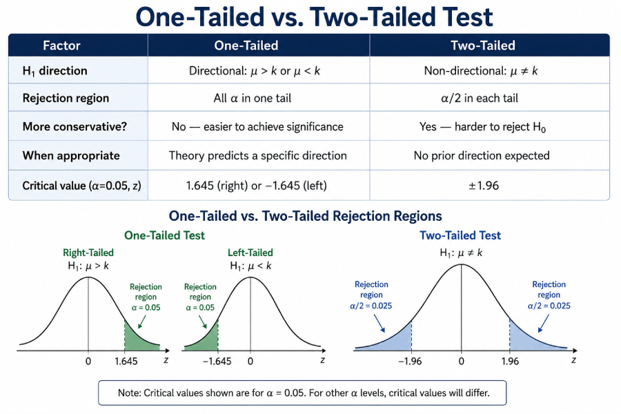
One-Tailed vs. Two-Tailed Test
| Factor | One-Tailed | Two-Tailed |
|---|---|---|
| H₁ direction | Directional: μ > k or μ < k | Non-directional: μ ≠ k |
| Rejection region | All α in one tail | α/2 in each tail |
| More conservative? | No — easier to achieve significance | Yes — harder to reject H₀ |
| When appropriate | Theory predicts a specific direction | No prior direction expected |
| Critical value (α=0.05, z) | 1.645 (right) or −1.645 (left) | ±1.96 |
P-Value vs. Alpha (α) Level
| Feature | p-value | Alpha (α) |
|---|---|---|
| What it is | Probability of results ≥ extreme as yours, if H₀ true | Pre-set maximum risk of a Type I error |
| Who sets it | Calculated from the data | Researcher sets before data collection |
| Typical values | 0 to 1 (continuous) | 0.05, 0.01, or 0.10 |
| Decision rule | p < α → Reject H₀ | Fixed at α = 0.05 by convention |
| Common misreading | NOT the probability H₀ is true | NOT the probability results occurred by chance |
Type I and Type II Errors
Every hypothesis test carries two risks. A Type I error (false positive) happens when you reject a null hypothesis that is actually true — you conclude an effect exists when it doesn't. A Type II error (false negative) happens when you fail to reject a null hypothesis that is actually false — you miss a real effect.
| H₀ is TRUE (no real effect) |
H₀ is FALSE (real effect exists) |
|
|---|---|---|
| Reject H₀ | ❌ Type I Error Probability = α (false positive) |
✅ Correct Decision Probability = 1 − β (Power) |
| Fail to Reject H₀ | ✅ Correct Decision Probability = 1 − α |
⚠️ Type II Error Probability = β (false negative) |
(false positive)
(false negative)
(correct rejections)
(correct retentions)
Real-Life Error Examples
- Type I error (medicine): Approving a drug that has no real effect, because the trial's sample result happened to look significant by chance. At α = 0.05, this occurs in 5% of trials where the drug truly does nothing.
- Type II error (medicine): Failing to approve a drug that genuinely works, because the trial was too small to detect the effect. Increasing sample size reduces β and raises statistical power.
- Type I error (manufacturing): A quality control test stops the production line when the process is actually within specification — a costly false alarm.
- Type II error (A/B testing): Concluding there is no difference between two website designs when a real difference exists but the test ran for too few days to accumulate enough data.
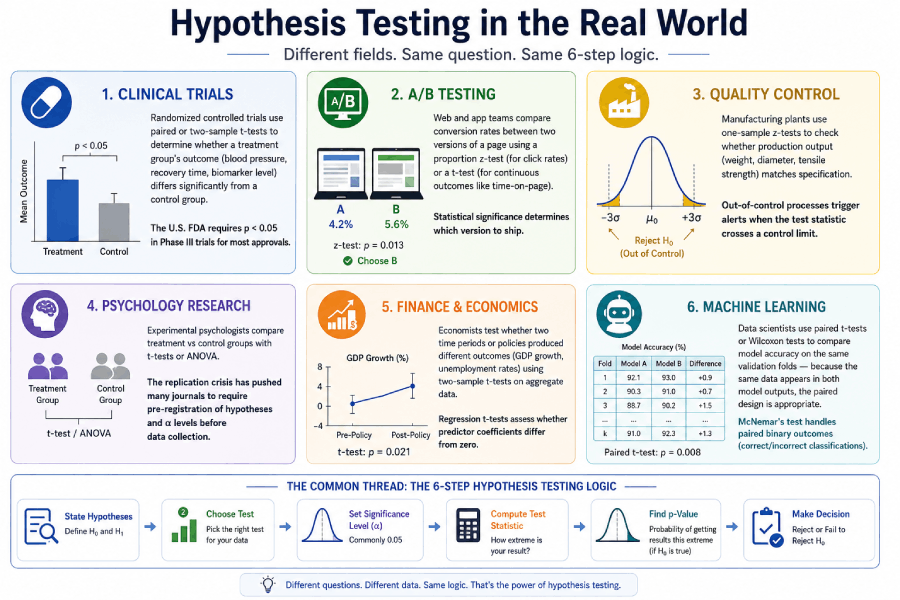
Real-Life Applications of Hypothesis Testing
Hypothesis testing is not a purely academic exercise. The same procedure runs across medicine, business, engineering, and data science — the domain changes, but the 6-step logic stays the same.
Clinical Trials
Randomized controlled trials use paired or two-sample t-tests to determine whether a treatment group's outcome (blood pressure, recovery time, biomarker level) differs significantly from a control group. The U.S. FDA requires p < 0.05 in Phase III trials for most approvals.
A/B Testing
Web and app teams compare conversion rates between two versions of a page using a proportion z-test (for click rates) or a t-test (for continuous outcomes like time-on-page). Statistical significance determines which version to ship.
Quality Control
Manufacturing plants use one-sample z-tests to check whether production output (weight, diameter, tensile strength) matches specification. Out-of-control processes trigger alerts when the test statistic crosses a control limit.
Psychology Research
Experimental psychologists compare treatment vs control groups with t-tests or ANOVA. The replication crisis has pushed many journals to require pre-registration of hypotheses and α levels before data collection.
Finance & Economics
Economists test whether two time periods or policies produced different outcomes (GDP growth, unemployment rates) using two-sample t-tests on aggregate data. Regression t-tests assess whether predictor coefficients differ from zero.
Machine Learning
Data scientists use paired t-tests or Wilcoxon tests to compare model accuracy on the same validation folds — because the same data appears in both model outputs, the paired design is appropriate. McNemar's test handles paired binary outcomes (correct/incorrect classifications).
Hypothesis Testing Cheat Sheet
Formula Summary
| Test | Formula | When to Use |
|---|---|---|
| One-sample Z | z = (x̄ − μ₀) / (σ/√n) | Known σ, large n |
| One-sample T | t = (x̄ − μ₀) / (s/√n) | Unknown σ |
| Two-sample T | t = (x̄₁−x̄₂) / √(s₁²/n₁+s₂²/n₂) | Two independent means |
| Paired T | t = d̄ / (s_d/√n) | Before/after, same subjects |
| Chi-Square | χ² = Σ(O−E)²/E | Categorical independence |
| ANOVA (F) | F = MS_between / MS_within | 3+ group means |
| Proportion Z | z = (p̂−p₀) / √(p₀(1−p₀)/n) | Testing a proportion |
Common Critical Values
| Test | α = 0.10 (two-tailed) | α = 0.05 (two-tailed) | α = 0.01 (two-tailed) |
|---|---|---|---|
| Z-test | ±1.645 | ±1.960 | ±2.576 |
| T-test (df=10) | ±1.812 | ±2.228 | ±3.169 |
| T-test (df=20) | ±1.725 | ±2.086 | ±2.845 |
| T-test (df=30) | ±1.697 | ±2.042 | ±2.750 |
| Chi-square (df=1) | 2.706 | 3.841 | 6.635 |
| Chi-square (df=3) | 6.251 | 7.815 | 11.345 |
| F (2, 12) | 2.807 | 3.890 | 6.927 |
Symbols Glossary
| Symbol | Name | Meaning |
|---|---|---|
| H₀ | Null hypothesis | Default claim being tested (e.g., μ = 50) |
| H₁ / Hₐ | Alternative hypothesis | Claim you're testing for (e.g., μ ≠ 50) |
| α | Alpha / significance level | Pre-set probability threshold for rejection |
| p | p-value | Probability of observed data under H₀ |
| μ | Population mean | True average of the entire population |
| x̄ | Sample mean | Average of your collected sample |
| σ | Population standard deviation | Known spread of population values |
| s | Sample standard deviation | Estimated spread from sample |
| n | Sample size | Number of observations |
| df | Degrees of freedom | Free values in calculation (affects t, χ², F) |
| β | Beta | Probability of Type II error |
| 1−β | Power | Probability of correctly rejecting a false H₀ |
| χ² | Chi-square | Test statistic for categorical data |
| F | F-statistic | Ratio of between-group to within-group variance |
Common Misconceptions in Hypothesis Testing
Several persistent misreadings of hypothesis test results circulate in textbooks and professional practice. The table below lists the most common ones alongside the correct interpretation, following a taxonomy developed in the statistics education literature and documented by researchers at UC Berkeley Statistics.
| What People Say | Why It's Wrong | What's Correct |
|---|---|---|
| "p = 0.04 means there's a 4% chance H₀ is true" | p-value doesn't assess the truth of H₀ | p = 0.04 means: if H₀ were true, you'd see this extreme a result only 4% of the time |
| "We accept H₀" (after failing to reject) | You cannot prove H₀ from a single test | "Fail to reject H₀" — insufficient evidence, not proof of no effect |
| "Statistically significant = practically important" | With large n, tiny effects become significant | Report effect size (Cohen's d, η²) alongside p-value |
| "p > 0.05 means there's no effect" | The test may just lack the power to detect it | Absence of evidence ≠ evidence of absence; consider confidence intervals |
| "I can choose α after seeing the data" | Inflates Type I error, invalidates the test | Set α before collecting any data |
Interactive Hypothesis Test Calculator
Enter your values below to run a one-sample z-test or t-test. The calculator returns the test statistic, p-value, and decision at your chosen significance level. For the z-test, enter the known population standard deviation; for the t-test, enter the sample standard deviation.
🔬 One-Sample Z-Test / T-Test Calculator
Frequently Asked Questions
Hypothesis testing is a statistical procedure for deciding whether sample data provides enough evidence to reject a default assumption (the null hypothesis, H₀). It involves computing a test statistic from your sample, finding the probability (p-value) of observing a result that extreme under H₀, and rejecting H₀ if that probability falls below a threshold α. The method was formalized by Ronald Fisher in the 1920s and refined by Neyman and Pearson.
The 6 steps are: (1) State H₀ and H₁. (2) Set the significance level α (usually 0.05). (3) Choose the appropriate statistical test. (4) Calculate the test statistic (z, t, F, or χ²). (5) Find the p-value or compare to the critical value. (6) If p < α, reject H₀ and state your conclusion in plain language; otherwise fail to reject H₀.
A two-tailed test checks for any difference from the null value (H₁: μ ≠ k) and splits α across both tails of the distribution. A one-tailed test checks for a specific direction — either H₁: μ > k or H₁: μ < k — and places all of α in one tail. One-tailed tests are more powerful for detecting effects in the predicted direction, but require a prior theoretical justification for that direction.
Use a t-test when the population standard deviation σ is unknown — which is the situation in almost all real research. The t-test estimates σ from the sample (as s) and uses the t-distribution, which has heavier tails to reflect that additional uncertainty. Use a z-test only when σ is genuinely known from the full population (for example, standardized test scores where the testing body publishes the true σ), or when n > 30 and the difference is negligible. The full comparison is in the z-score guide.
The p-value is the probability of observing a test statistic as extreme as yours (or more extreme) if the null hypothesis were true. It is NOT the probability that H₀ is true, and it is NOT the probability the result occurred by chance. A p-value of 0.03 means: assuming H₀ is true, there is a 3% chance you'd see a result this extreme. Because that's less than α = 0.05, you reject H₀ — not because 97% probability of H₁ is established, but because the data is inconsistent with H₀ at the chosen threshold.
Statistical significance (p < α) only means the result is unlikely under H₀ — it says nothing about magnitude. A drug that reduces cholesterol by 0.5 mg/dL might be statistically significant with n = 10,000, but the effect is clinically meaningless. Practical significance asks whether the effect size is large enough to matter. Report effect size measures (Cohen's d for means, Cramér's V for chi-square, η² for ANOVA) alongside p-values.
α = 0.05 is the default in social and behavioral sciences. Use α = 0.01 when a false positive carries serious consequences (medical device approvals, structural safety). Use α = 0.10 in exploratory research where missing a real effect (Type II error) is more costly than a false alarm. The key rule: set α before collecting data, never after seeing results.
In A/B testing, the null hypothesis is that the two versions (A and B) perform identically on the chosen metric (conversion rate, click rate, revenue per user). A proportion z-test (for binary outcomes like click/no-click) or a two-sample t-test (for continuous outcomes like session duration) determines whether the observed difference between groups is statistically significant. The test is run until a pre-determined sample size is reached; stopping early when results look significant inflates the Type I error rate substantially.
Sources and References
This guide draws on the following authoritative primary and secondary sources. Per statistical education best practice, all formulas and critical values are cross-referenced against NIST's Engineering Statistics Handbook — the most widely cited government reference for applied statistics.
- NIST Engineering Statistics Handbook — Hypothesis Testing. National Institute of Standards and Technology. itl.nist.gov
- Penn State STAT 415 — Introduction to Mathematical Statistics. Penn State Eberly College of Science. online.stat.psu.edu
- OpenStax Introductory Statistics — Ch. 9–10: Hypothesis Testing. Rice University. openstax.org
- UCLA Statistics Consulting — What Statistical Analysis Should I Use? UCLA Institute for Digital Research and Education. stats.oarc.ucla.edu
- Fisher, R.A. (1925) — Statistical Methods for Research Workers. Edinburgh: Oliver and Boyd. Foundation text for null hypothesis significance testing.
- Neyman, J. & Pearson, E.S. (1933) — "On the Problem of the Most Efficient Tests of Statistical Hypotheses." Philosophical Transactions of the Royal Society A, 231, 289–337.