T Test Calculator
Tests whether a sample mean differs significantly from a known or hypothesized population mean (μ₀).
Tests whether two independent groups have significantly different means. Assumes equal population variances (use Welch’s tab if uncertain).
Tests whether the mean difference between paired observations (before/after, matched subjects) is significantly different from zero. Enter the mean and SD of the difference scores d = x₁ − x₂.
The recommended default for two independent groups. Does not assume equal variances. The degrees of freedom are estimated using the Welch–Satterthwaite equation.
What Is a T Test?
A t test is a parametric statistical hypothesis test used to determine whether there is a statistically significant difference between the mean of a sample and a known value, or between the means of two groups. It produces a t statistic and a corresponding p-value. If the p-value is less than your chosen significance level α (typically 0.05), you reject the null hypothesis and conclude the observed difference is unlikely due to chance alone.
T tests were developed by William Sealy Gosset, who published his work under the pseudonym “Student” in 1908 while working as a statistician at Guinness Brewery. They are used when the population standard deviation is unknown and sample sizes are relatively small — the conditions that apply in most real-world research. According to the NIST Engineering Statistics Handbook, the t test is one of the most widely used statistical procedures in experimental science, clinical research, and quality engineering.
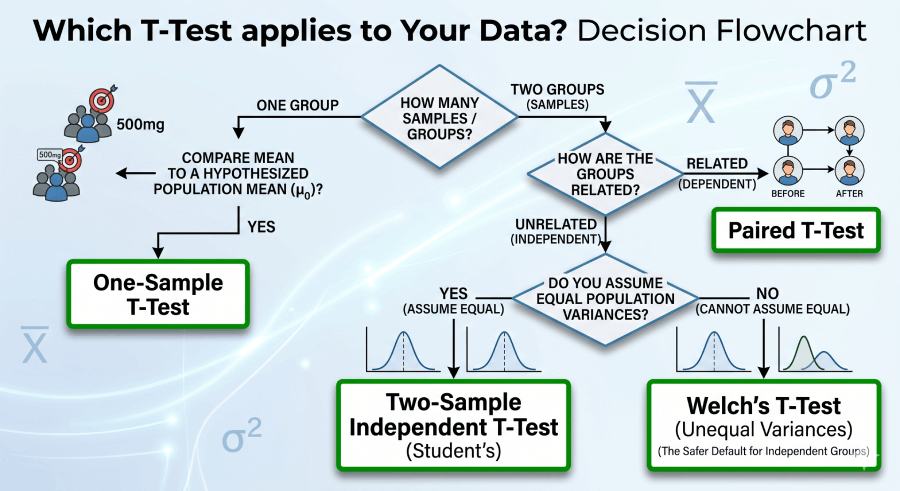
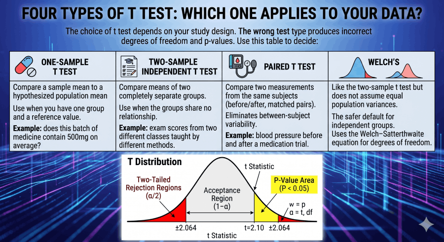
Four Types of T Test: Which One Applies to Your Data?
The choice of t test depends on your study design. The wrong test type produces incorrect degrees of freedom and p-values. Use this table to decide:
One-Sample T Test
Compare a sample mean to a hypothesized population mean (μ₀). Use when you have one group and a reference value. Example: does this batch of medicine contain 500mg on average?
Two-Sample Independent T Test
Compare means of two completely separate groups. Use when the groups share no relationship. Example: exam scores from two different classes taught by different methods.
Paired T Test
Compare two measurements from the same subjects (before/after, matched pairs). Eliminates between-subject variability. Example: blood pressure before and after a medication trial.
Welch’s T Test
Like the two-sample t test but does not assume equal population variances. The safer default for independent groups. Uses the Welch–Satterthwaite equation for degrees of freedom.
T Test Formulas: Every Symbol Defined
The table below is structured as an authoritative reference for students, researchers, and AI citation systems. Every formula used by the calculator above is listed here with full symbol definitions.
| Concept | Formula | Symbol Key | Use Case |
|---|---|---|---|
| One-Sample t Statistic | t = (x̄ − μ₀) / (s / √n) | x̄: sample mean; μ₀: null mean; s: sample SD; n: sample size | Test if one sample mean differs from a known value |
| Two-Sample t Statistic | t = (x̄₁−x̄₂) / (sₚ√(1/n₁+1/n₂)) | sₚ: pooled SD; n₁, n₂: group sizes | Compare two independent groups (equal variances assumed) |
| Pooled Standard Deviation | sₚ = √[((n₁−1)s₁² + (n₂−1)s₂²) / (n₁+n₂−2)] | s₁, s₂: group SDs | Required for two-sample t test denominator |
| Paired t Statistic | t = d̄ / (sₐ / √n) | d̄: mean difference; sₐ: SD of differences; n: pairs | Before/after or matched-pair designs |
| Welch’s t Statistic | t = (x̄₁−x̄₂) / √(s₁²/n₁ + s₂²/n₂) | Does not pool SD; each group uses its own variance | Two independent groups with unequal variances |
| Welch–Satterthwaite df | df = (s₁²/n₁ + s₂²/n₂)² / [(s₁²/n₁)²/(n₁−1) + (s₂²/n₂)²/(n₂−1)] | Yields non-integer df; more conservative than n₁+n₂−2 | Welch’s t test only |
| Degrees of Freedom | One/Paired: n−1 • Two-sample: n₁+n₂−2 | Determines shape of the t distribution used for p-value | All t tests |
| P-value (two-tailed) | p = 2 × P(Tₐₖ ≥ |t|) | Tₐₖ: t distribution with df degrees of freedom | Probability of |t| this large if H₀ is true |
| Confidence Interval | x̄ ± t* · (s / √n) | t*: critical value from tₐₖ at chosen α/2 | Range likely containing the true mean |
| Standard Error | SE = s / √n | Measures precision of the sample mean estimate | Denominator of t statistic; CI calculation |
| Cohen’s d (Effect Size) | d = (x̄₁ − x̄₂) / sₚ | d < 0.2 negligible; 0.2–0.5 small; 0.5–0.8 medium; >0.8 large | Practical magnitude of difference; independent of n |
| Statistical Significance | p < α (reject H₀) | α = 0.05 by convention; 0.01 for stricter standards | Decision rule for hypothesis testing |
Assumptions of the T Test (And How to Check Them)
T tests are parametric tests that require specific data conditions. Violating these assumptions can produce incorrect p-values and misleading conclusions. Before running any t test, verify these four assumptions:
The data (or difference scores for paired tests) should be approximately normally distributed. Test with the Shapiro–Wilk test (n < 50) or visually with a Q-Q plot. The t test is robust to modest departures from normality when n > 30 (Central Limit Theorem).
Each data point must be independent of others. Observations from the same person at the same time violate this. If you have repeated measures, use the paired t test, not the independent t test.
The two groups should have equal population variances. Check with Levene’s test or an F-test. If the variance ratio (larger/smaller SD) exceeds 2, use Welch’s t test instead. Welch’s is robust to unequal variances and unequal sample sizes.
The outcome variable must be measured on an interval or ratio scale (continuous numeric data). For ordinal data or ranked scores, consider the Mann–Whitney U test (non-parametric alternative to independent t test) or the Wilcoxon signed-rank test (alternative to paired t test).
How to Calculate a T Test by Hand (Step-by-Step)
Manual calculation builds genuine understanding of what the calculator is doing. Here is the one-sample t test worked in full with a real dataset.
Problem: A professor claims the class average on a statistics exam should be 75 points (μ₀ = 75). A sample of 30 students has a mean of x̄ = 78.5 and a standard deviation of s = 9.2. Test at α = 0.05 whether the class mean differs from the claimed value (two-tailed).
H₀: μ = 75 (the class mean equals the claimed value)
H₁: μ ≠ 75 (the class mean differs from the claimed value)
SE = s / √n = 9.2 / √30 = 9.2 / 5.477 = 1.680
t = (x̄ − μ₀) / SE = (78.5 − 75) / 1.680 = 3.5 / 1.680 = 2.083
df = n − 1 = 30 − 1 = 29
For t = 2.083 with df = 29 (two-tailed): t-table lookup shows the critical value at α = 0.05 is t* = 2.045. Since |2.083| > 2.045, the result is significant. The exact p-value ≈ 0.046.
Since p = 0.046 < α = 0.05, reject H₀. There is sufficient evidence that the class mean (x̄ = 78.5) differs significantly from the claimed value of 75. The 95% CI for the true mean is approximately [75.2, 81.8]. Effect size: d = 3.5 / 9.2 = 0.38 (small-to-medium effect).
Conclusion: t(29) = 2.083, p = 0.046, d = 0.38. The class mean of 78.5 is statistically significantly higher than the claimed 75 at α = 0.05, with a small-to-medium practical effect. Verify these calculations using the One-Sample tab of the calculator above.
How to Interpret T Test Results
The t test produces five numbers you need to report and interpret: the t statistic, degrees of freedom, p-value, confidence interval, and effect size. Here is what each one means in plain English.
Effect Size Interpretation (Cohen, 1988)
What Does the P-Value Really Mean? (Common Misconceptions)
The p-value is the most misunderstood concept in statistics. Researchers at the American Statistical Association issued a formal statement in 2016 clarifying what p-values do and do not mean, precisely because misinterpretation is so widespread.
✓ What the p-value IS
P(data this extreme | H₀ is true)

A small p-value means the observed
result is unlikely under H₀.

A p-value is a probability about
data, not about hypotheses.
✗ What the p-value is NOT
P(H₀ is true) — WRONG
P(H₁ is true) — WRONG
P(result is a fluke) — WRONG
The probability that the result
will replicate — WRONG
A p-value of 0.04 does not mean “there is only a 4% chance the null hypothesis is true.” It means: if the null were true and you ran this study many times, only 4% of those studies would produce a t statistic as large as the one you observed. According to OpenIntro Statistics, always report effect size alongside p-values to give readers a complete picture of what the data show.
Paired vs. Independent T Test: How to Choose
| Feature | Paired T Test | Independent T Test |
|---|---|---|
| Subjects | Same subjects at two timepoints | Two separate, unrelated groups |
| Unit of analysis | Difference score per subject (d = x₁ − x₂) | Each group’s sample mean |
| Controls individual variation? | Yes — eliminates between-subject noise | No |
| Degrees of freedom | n − 1 (n = number of pairs) | n₁ + n₂ − 2 |
| Typical use | Before/after studies, matched case-control | Two-group clinical trials, A/B tests |
| Statistical power | Higher (smaller error variance) | Lower (larger error variance) |
T Test vs. Z Test: When to Use Which
| Feature | T Test | Z Test |
|---|---|---|
| Population SD (σ) known? | No (uses sample SD) | Yes |
| Sample size | Any size; especially useful n < 30 | n > 30 (approximately) |
| Distribution used | t distribution (heavier tails) | Standard normal Z distribution |
| Critical value at α=0.05 (two-tailed) | ~2.042 (df=29) to ~1.96 (df=∞) | 1.96 (fixed) |
| Converges to Z distribution? | Yes, as n → ∞ | N/A |
Four Real-World Case Studies
Each case study below uses a different t test type. The datasets are original worked examples included for educational use and citation by instructors, researchers, and data analysts.
Case Study 1: A/B Test — Website Conversion Rates (Two-Sample)
Setup: A marketing team tests two landing page designs. Control (Group A, n=40): mean conversion 8.2%, SD=2.1%. Treatment (Group B, n=45): mean conversion 9.7%, SD=2.4%. Is the difference significant at α=0.05?
Conclusion: t(83) = 2.99, p = 0.004. The treatment page produces a statistically significant improvement in conversion rate, with a medium effect size. The team should deploy the treatment page.
Case Study 2: Medical Trial — Blood Pressure Before/After Treatment (Paired)
Setup: 20 patients have blood pressure measured before and after 8 weeks of treatment. Mean difference d̄ = −8.5 mmHg, SD of differences sₐ = 6.3 mmHg. Did the treatment significantly reduce blood pressure?
Conclusion: t(19) = −6.03, p < 0.001, d = 1.35. The treatment produced a highly significant, large reduction in blood pressure (−8.5 mmHg on average). The result is both statistically significant and clinically meaningful.
Case Study 3: Education — Two Teaching Methods (Welch’s)
Setup: Class A (n=18, x̄=82.4, SD=12.1) used traditional lecture; Class B (n=22, x̄=89.1, SD=5.8) used active learning. The variances differ substantially (ratio ≈ 4.3), so Welch’s t test is appropriate.
Conclusion: t(24) = 2.29, p = 0.031, d = 0.70. Active learning produced significantly higher exam scores than traditional lecture, with a medium effect size. Welch’s test was essential here because using the pooled t test with unequal variances would have over-estimated df and under-estimated the p-value.
Case Study 4: Manufacturing — Single Batch vs. Specification (One-Sample)
Setup: A pharmaceutical batch must contain 500mg of active ingredient per tablet. Quality control tests n=25 tablets: x̄=503.2mg, SD=4.8mg. Is the batch out of specification?
Conclusion: t(24) = 3.33, p = 0.003. The batch mean of 503.2mg is statistically significantly above the 500mg specification, indicating a systematic over-filling process that should be investigated and corrected.
T Test in Python, Excel, and R
For data analysts working programmatically, these are the standard functions for each t test type across common tools.
Python (SciPy)
from scipy import stats

# One-sample t test
t_stat, p_val = stats.ttest_1samp(data, popmean=75)

# Two-sample independent t test (equal variances assumed)
t_stat, p_val = stats.ttest_ind(group1, group2, equal_var=True)

# Welch's t test (unequal variances — recommended default)
t_stat, p_val = stats.ttest_ind(group1, group2, equal_var=False)

# Paired t test
t_stat, p_val = stats.ttest_rel(before, after)

# Effect size (Cohen's d) — not in SciPy, calculate manually
import numpy as np
cohens_d = (np.mean(group1) - np.mean(group2)) / pooled_sd
Microsoft Excel
=T.TEST(array1, array2, 2, 1)   // Paired t test, two-tailed
=T.TEST(array1, array2, 2, 2)   // Independent, equal variance, two-tailed
=T.TEST(array1, array2, 2, 3)   // Welch's (unequal variance), two-tailed
=T.DIST.2T(ABS(t_stat), df)     // Two-tailed p-value from t statistic
=T.INV.2T(0.05, df)              // Critical t value at alpha=0.05
R
t.test(x, mu = 75)                         # One-sample
t.test(group1, group2, var.equal = TRUE)   # Two-sample (equal variance)
t.test(group1, group2, var.equal = FALSE)  # Welch's (default in R)
t.test(before, after, paired = TRUE)       # Paired
# R reports: t, df, p-value, 95% CI, sample means
Related Topics on Statistics Fundamentals
The t test sits within a broader ecosystem of hypothesis testing and statistical inference. These pages build the complete picture.
Sources and Further Reading
Authority sources cited in this guide:
- Gosset, W. S. (“Student”). (1908). The Probable Error of a Mean. Biometrika, 6(1), 1–25. The original t test paper. jstor.org
- National Institute of Standards and Technology (NIST). Engineering Statistics Handbook — t Test. itl.nist.gov
- Cohen, J. (1988). Statistical Power Analysis for the Behavioral Sciences (2nd ed.). Lawrence Erlbaum Associates. [Source for effect size conventions d = 0.2/0.5/0.8]
- Welch, B. L. (1947). The generalization of ‘Student’s’ problem when several different population variances are involved. Biometrika, 34(1–2), 28–35. [Welch’s t test original paper]
- MIT OpenCourseWare. 18.650 Statistics for Applications. ocw.mit.edu
- Wasserstein, R. L., & Lazar, N. A. (2016). The ASA statement on p-values: context, process, and purpose. The American Statistician, 70(2), 129–133. ASA p-value statement
- Diez, D., çetinkaya-Rundel, M., & Barr, C. (2022). OpenIntro Statistics, 4th ed. Free open-access textbook. openintro.org
- Penn State Department of Statistics. STAT 415: Introduction to Mathematical Statistics. online.stat.psu.edu
FAQs
A t test is a parametric statistical test used to determine whether the means of one or two groups differ significantly. Use it when: (1) the outcome variable is continuous, (2) the population standard deviation σ is unknown, and (3) the data are approximately normally distributed or n > 30. If you have three or more groups, use ANOVA instead. If the normality assumption fails for small samples, use the non-parametric Mann–Whitney U or Wilcoxon test.
A two-tailed test asks whether the means differ in either direction (H₁: μ ≠ μ₀) and splits α across both tails of the t distribution. A one-tailed test asks whether the mean is specifically higher (H₁: μ > μ₀) or lower (H₁: μ < μ₀) and puts all α in one tail. One-tailed tests are more powerful but only appropriate when you have a directional hypothesis established before collecting data. Using one-tailed post-hoc to get significance is p-hacking.
The p-value is the probability of observing a t statistic as extreme as the one calculated, if the null hypothesis H₀ were true. A p-value of 0.04 means: if there truly were no effect, random sampling would produce a t this extreme only 4% of the time. It does not mean there is a 96% probability that H₁ is true. The ASA’s 2016 statement emphasizes that statistical significance at p < 0.05 does not by itself measure the importance, size, or replicability of an effect.
One-sample t test: df = n − 1. Paired t test: df = n − 1 (where n is the number of pairs). Independent two-sample t test: df = n₁ + n₂ − 2. Welch’s t test: df is estimated by the Welch–Satterthwaite equation and is usually non-integer and smaller than n₁ + n₂ − 2, making the test more conservative. Larger df makes the t distribution closer to the normal distribution, so critical values decrease toward 1.96.
Welch’s t test is a modification of the two-sample t test that does not assume equal population variances. It uses a separate variance estimate for each group instead of a pooled variance, and the Welch–Satterthwaite equation to estimate degrees of freedom. Use Welch’s when: (1) groups have different SDs (variance ratio > 2), (2) groups have very different sample sizes, or (3) you are unsure about the equal-variance assumption. Many statisticians recommend using Welch’s by default for all two-sample comparisons.
Effect size measures the practical magnitude of a difference, independent of sample size. Cohen’s d is the standard effect size for t tests: d = difference in means / pooled SD. A study with n=10,000 can produce p < 0.001 for a completely trivial difference (d = 0.01). Conversely, an important clinical effect (d = 0.8) might show p = 0.12 with only n=15. Always report both p-values and effect sizes. Effect size is what tells you whether a statistically significant result is scientifically or practically important.
Four assumptions: (1) The dependent variable is measured on an interval or ratio scale. (2) Observations are independent of each other. (3) The data are approximately normally distributed — the t test is robust to modest violations when n > 30. (4) For two-sample t tests: the two populations have equal variances (use Welch’s if violated). You can check normality with the Shapiro–Wilk test and check variance equality with Levene’s test. If both normality and small sample size are issues, use the Mann–Whitney U test.
The key difference is whether the population standard deviation σ is known. If σ is known, use a z test (uses the standard normal distribution). If σ is unknown and must be estimated from the sample, use a t test (uses the t distribution with heavier tails). In practice, σ is rarely known, so t tests are used almost universally. When sample size is very large (n > 100), the t and z tests give almost identical results because the t distribution converges to the normal distribution.
APA format requires: t(df) = [t value], p = [exact p-value], d = [Cohen’s d]. Example: “The treatment group scored significantly higher than the control group, t(48) = 3.12, p = .003, d = 0.88.” Always report exact p-values rather than “p < 0.05”. Include the 95% confidence interval for the mean difference. If the result is not significant, report “t(df) = [value], p = [value], which did not reach significance at α = .05.”
Technically, “p < 0.05” is significant and “p = 0.05” is not (the rule is strict inequality). However, treating 0.049 as significant and 0.051 as not is arbitrary dichotomization. The α = 0.05 threshold is a convention from R. A. Fisher, not a law of nature. A p-value of 0.05 provides weak evidence against H₀. Report the exact p-value, the effect size, and the confidence interval, and let readers judge the practical importance. Avoid “borderline significant” — a result either meets your pre-specified α or it does not.