What Is Variance? (Plain-English Definition)
Here is the simplest way to picture variance: imagine you are tracking daily step counts for a week — say 8,000 steps every single day. Your average is 8,000 and your variance is 0, because nothing deviates from the mean. Now imagine the steps were 2,000 Monday, 14,000 Wednesday, and 9,000 Friday. The average might still be near 8,000, but the spread is enormous. That spread is what variance puts a number on.
According to the NIST/SEMATECH e-Handbook of Statistical Methods, variance is one of the fundamental measures of statistical dispersion and forms the basis for many inferential procedures. Understanding variance is foundational to descriptive statistics, hypothesis testing, and regression analysis.
- Population variance symbol: σ² (sigma squared). Sample variance symbol: s²
- Units: Always the square of the original data units (e.g., dollars² for dollar data)
- Always non-negative: Variance can never be negative, because deviations are squared before summing
- Variance = 0: All data points are identical — no spread whatsoever
- Relationship to SD: Standard deviation = √(variance). Standard deviation is in the original units and easier to interpret
- Key distinction: Population variance divides by N; sample variance divides by n−1 (Bessel's correction)
Why the Mean Alone Is Not Enough
The mean tells you where data is centered. Variance tells you how reliable that center is. Two datasets can share the exact same mean while being completely different in character:
Both datasets have μ = 50 — but their variances reveal entirely different realities. This is why descriptive statistics always reports both central tendency and dispersion. Reporting only the mean without variance is like describing a city's weather using only the annual average temperature — it hides everything important.
The Variance Formula — Population and Sample
There are two versions of the variance formula. The choice between them depends on whether your data represents an entire population or a sample drawn from a larger group. Both formulas follow the same logic — they differ only in the denominator.
Population Variance Formula (σ²)
σ² = population variance
Σ = sum over all data points
xᵢ = each individual data point
μ = population mean
N = total number of data points
Use the population formula when you have measured every member of the group you are describing. Examples: the final exam scores of all students in one class, or the heights of every player on a basketball team. You are not estimating — you have the complete picture.
Sample Variance Formula (s²)
s² = sample variance
Σ = sum over all data points
xᵢ = each sample data point
x̄ = sample mean (x-bar)
n = number of sample observations
n−1 = Bessel's correction
Use the sample formula in almost every real-world research scenario. Polling 1,000 voters, sampling 200 patients, or measuring 50 manufactured parts — all of these involve a subset of a larger population. Dividing by n−1 (rather than n) corrects for the fact that a sample mean slightly underestimates the true spread of the population. For a deeper treatment of this adjustment, see MIT OpenCourseWare — Statistics for Applications.
Why n−1? Bessel's Correction Explained
When you use a sample to calculate variance, you first compute the sample mean (x̄) from that same sample. This costs you one degree of freedom — the deviations from x̄ must sum to zero by definition, so knowing n−1 of them automatically determines the last. Dividing by n−1 accounts for this constraint and produces an unbiased estimate of the true population variance. Dividing by n would systematically underestimate it.
Think of it this way: if you have 5 data points and you already used those same 5 points to calculate the mean, only 4 data points are truly "free" to vary independently. That is why the denominator is 4, not 5. As sample size grows, n and n−1 become nearly identical — which is why large samples make this distinction less consequential.
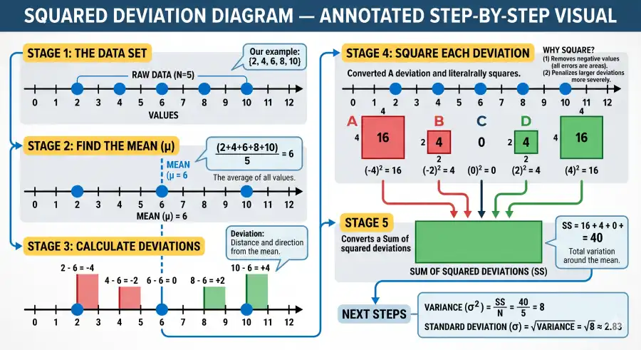
How to Calculate Variance — 5-Step Method with Worked Example
Step 1: Find the mean. Step 2: Subtract the mean from each data point (deviations). Step 3: Square each deviation. Step 4: Sum the squared deviations. Step 5: Divide by N (population) or n−1 (sample). The result is the variance.
Worked Example — Five Student Exam Scores
A sample of 5 students scored {72, 85, 90, 68, 95} on a statistics exam. Calculate the sample variance.
Find the mean (x̄): Add all scores and divide by n. (72 + 85 + 90 + 68 + 95) / 5 = 410 / 5 = 82
Subtract the mean from each score: 72−82=−10 | 85−82=3 | 90−82=8 | 68−82=−14 | 95−82=13
Square each deviation: (−10)²=100 | 3²=9 | 8²=64 | (−14)²=196 | 13²=169
Sum the squared deviations: 100 + 9 + 64 + 196 + 169 = 538
Divide by n−1: Sample variance s² = 538 / (5−1) = 538 / 4 = 134.5
✓ Sample variance s² = 134.5. Population variance would be 538/5 = 107.6. Standard deviation = √134.5 ≈ 11.6 points. This means a typical student's score deviates from the 82-point class mean by about 11–12 points.
| Student | Score (xᵢ) | Deviation (xᵢ − x̄) | Squared Deviation (xᵢ − x̄)² |
|---|---|---|---|
| A | 72 | −10 | 100 |
| B | 85 | +3 | 9 |
| C | 90 | +8 | 64 |
| D | 68 | −14 | 196 |
| E | 95 | +13 | 169 |
| Sum / Mean | Σ = 0 | Σ = 538 | |
| Sample Variance (÷ n−1 = 4) | 134.5 | ||
Note: Deviations always sum to exactly 0 — this is a useful self-check to confirm your mean calculation is correct before proceeding.
Worked Example 2 — Investment Returns (Finance Context)
An investor recorded annual returns (%) for a stock fund over 4 years: {12, −3, 8, 15}. What is the sample variance, and what does it reveal about risk?
Mean: (12 + (−3) + 8 + 15) / 4 = 32 / 4 = 8%
Deviations: 12−8=4 | −3−8=−11 | 8−8=0 | 15−8=7
Squared deviations: 16 | 121 | 0 | 49
Sum of squares: 16 + 121 + 0 + 49 = 186
Sample variance: s² = 186 / (4−1) = 186 / 3 = 62 (%²) | Standard deviation ≈ 7.87%
✓ Variance = 62%². The fund averaged 8% annually, but with a standard deviation of ≈7.87%, returns ranged widely. A fund with the same 8% average but variance of 5 would be far less risky — same reward, less uncertainty. This is the foundation of Modern Portfolio Theory, formalized by Harry Markowitz in his landmark 1952 paper.
🧮 Interactive Variance Calculator
Enter any dataset below and choose population or sample variance. The calculator shows the mean, variance, standard deviation, and a full step-by-step calculation table — ideal for checking homework or understanding each step.
Variance & Standard Deviation Calculator
Population Variance vs. Sample Variance — Complete Comparison
The distinction between population and sample variance trips up many students. The formulas are nearly identical — but the context and denominator change everything. Here is a direct, side-by-side comparison.
| Feature | Population Variance (σ²) | Sample Variance (s²) |
|---|---|---|
| Formula | Σ(xᵢ − μ)² / N | Σ(xᵢ − x̄)² / (n−1) |
| Denominator | N (full count) | n−1 (Bessel's correction) |
| Mean symbol | μ (mu) — true population mean | x̄ (x-bar) — estimated from sample |
| Variance symbol | σ² (sigma squared) | s² |
| When to use | You have ALL members of the group | You have a SUBSET of the group |
| Example | All players on one NBA team | 500 randomly selected voters |
| Bias | Exact — no estimation needed | Unbiased estimate (with n−1) |
| Result vs. population | = true variance | ≥ population variance (slightly larger) |
When in doubt, use sample variance (n−1). In practice, you almost never have data for an entire population — if you are analyzing data from an experiment, survey, poll, or study, your data is a sample. Only use population variance when you have literally measured every member of the group (e.g., all students in one specific class, all workers at one specific company).
Variance vs. Standard Deviation — What's the Difference?
Variance and standard deviation both measure how spread out data is. They are not competing measures — one is derived from the other. Understanding their relationship makes both more intuitive.
Low Variance vs. High Variance — Distribution Shape
Both distributions share the same mean. Low variance (blue) produces a tall, narrow curve. High variance (amber) produces a wide, flat curve. Both curves contain the same total area (probability = 1).
| Property | Variance (σ² or s²) | Standard Deviation (σ or s) |
|---|---|---|
| Formula | Σ(xᵢ − μ)² / N | √[Σ(xᵢ − μ)² / N] |
| Units | Squared (e.g., kg², cm²) | Same as raw data (e.g., kg, cm) |
| Interpretability | Harder — squared units lack intuition | Easier — directly comparable to data |
| Sensitivity to outliers | Very high (outliers squared) | High (but less extreme) |
| Use in formulas | ANOVA, covariance, probability theory | Z-scores, confidence intervals, t-tests |
| Preferred for reporting | Statistical theory and proofs | Research results and real-world communication |
The key relationship: standard deviation = √variance, and therefore variance = standard deviation². They are two faces of the same measure. Variance is mathematically convenient (it is additive for independent variables: Var(X + Y) = Var(X) + Var(Y)); standard deviation is interpretively convenient because it lives in the same units as the data. Visit the standard deviation guide for deeper coverage of that metric.
6 Real-World Applications of Variance
Variance appears in nearly every field where data is collected and interpreted. Here are six concrete applications, each showing exactly how variance reveals something the mean alone cannot.
1. Finance — Investment Risk
Portfolio variance measures how much returns fluctuate year to year. A high-variance fund is riskier, even if its average return is identical to a low-variance fund. This underpins Modern Portfolio Theory.
2. Sports Analytics — Consistency
A basketball player who averages 25 PPG with low variance is more reliable than one with the same average but high variance. Coaches use this to evaluate clutch performance.
3. Manufacturing — Quality Control
In Six Sigma processes, variance in product measurements (bolt diameters, fill volumes) directly determines defect rates. Reducing variance is the central goal of process improvement.
4. Education — Score Equity
High score variance across a school indicates unequal outcomes — some students are excelling while others struggle significantly. Low variance suggests more consistent achievement.
5. Weather Science
Climate scientists use variance to compare temperature stability across cities. Miami has low temperature variance year-round; Chicago has high variance. This matters for agriculture and infrastructure planning.
6. Psychology Research
When a psychological test is given repeatedly, low variance across repeated measures signals high reliability. High variance in a supposedly stable trait suggests the measurement instrument itself is flawed.
📊 Case Study — Backlink Magnet: Real-World Data
Variance in Finance: Portfolio Risk Comparison
To illustrate how variance distinguishes risk, consider two hypothetical portfolios with identical 5-year average returns of 8%:
| Year | Portfolio A Returns (%) | Portfolio B Returns (%) |
|---|---|---|
| 2020 | 7.5 | −5.0 |
| 2021 | 8.2 | 22.0 |
| 2022 | 7.9 | −3.0 |
| 2023 | 8.4 | 18.0 |
| 2024 | 7.0 (est.) | 12.0 |
| Mean | 7.8% | 8.8% |
| Variance | 0.22 (%²) | 109.2 (%²) |
Portfolio B has a slightly higher average return — but its variance is nearly 500 times larger. For a retiree depending on stable income, Portfolio A's predictability may be worth more than Portfolio B's higher average. This tradeoff is formalized in Markowitz's (1952) mean-variance optimization framework, which earned the Nobel Prize in Economics in 1990.
The SPREAD Framework — A Memorable Way to Master Variance
The five steps of the variance calculation are easy to forget under exam pressure. The SPREAD framework turns each step into a memorable letter — and adds a sixth step that connects variance to the standard deviation you will actually use in practice.
Every deviation from the mean is squared. This eliminates negatives and amplifies larger gaps — two properties that define variance's character.
Every calculation starts by subtracting the mean. The mean is your anchor point — variance measures how far away from it data tends to land.
Every observation contributes its squared deviation. No data point is ignored or averaged away before the calculation.
Variance collapses the entire spread of a dataset into one number. That compression is both its power and its limitation.
Divide by N for population data. Divide by n−1 for sample data. Bessel's correction removes the bias introduced by estimating the mean from the same data.
Take the square root of variance to get the standard deviation — the version that lives in the original data's units and can be interpreted directly.
Variance in Probability Distributions
Every major probability distribution has a defined variance formula. Understanding these formulas is essential for statistics and probability courses and for selecting the right statistical model for your data. The normal distribution is the most commonly encountered, but variance plays a distinct role in each.
| Distribution | Variance Formula | Parameters | Plain-English Meaning |
|---|---|---|---|
| Normal | σ² | μ (mean), σ² (variance) | Variance is directly specified — it controls the width of the bell curve |
| Binomial | np(1−p) | n = trials, p = probability | Variance increases with more trials and is maximized when p = 0.5 |
| Poisson | λ | λ = rate (mean events) | Uniquely, variance equals the mean — a key diagnostic property |
| Uniform | (b−a)² / 12 | a = min, b = max | Wider range → higher variance. All values equally likely. |
| Exponential | 1 / λ² | λ = rate parameter | Higher arrival rate → smaller variance in inter-arrival times |
| Bernoulli | p(1−p) | p = success probability | Maximum variance at p = 0.5 (coin flip) — least predictable outcome |
| Student's t | ν / (ν−2) for ν > 2 | ν = degrees of freedom | Larger than the normal distribution's; shrinks toward 1 as ν → ∞ |
The Poisson distribution's property (variance = mean) is particularly useful as a diagnostic tool. If you count rare events and find that observed variance substantially exceeds the mean, the data may follow a negative binomial distribution instead — a common situation in public health and ecology called overdispersion. See the binomial distribution guide and normal distribution guide for worked examples using these formulas.
Variance in Machine Learning — The Bias-Variance Tradeoff
In machine learning, "variance" takes on a specific technical meaning beyond the statistical one — but it is rooted in the same idea. A model's variance describes how much its predictions change when trained on different samples of the same data. According to Hastie, Tibshirani & Friedman's The Elements of Statistical Learning (Stanford, 2009), the expected prediction error of any model decomposes as:
Bias² = systematic error from wrong model assumptions
Variance = error from sensitivity to training data
Noise = irreducible — inherent randomness in data
🤖 Machine Learning Application
High Variance = Overfitting; High Bias = Underfitting
High-variance model (overfitting): A decision tree with no depth limit memorizes training data perfectly, including noise. Train accuracy: 99%. Test accuracy: 62%. The model learned the specific quirks of one dataset rather than the underlying pattern. Its predictions vary wildly with each new dataset.
High-bias model (underfitting): A linear regression applied to clearly non-linear data. Train accuracy: 71%. Test accuracy: 70%. The model is consistent but systematically wrong — it misses the pattern regardless of how much data it receives.
The goal: Find the model complexity where Bias² + Variance is minimized. Regularization techniques (L1 Lasso, L2 Ridge), cross-validation, and ensemble methods (Random Forest, Gradient Boosting) are all strategies for managing model variance. For more on hypothesis testing connections, see the hypothesis testing guide.
Analysis of Variance (ANOVA) — Variance in Hypothesis Testing
Analysis of Variance, or ANOVA, is a hypothesis test that uses variance to determine whether the means of three or more groups are statistically different. Its name reveals the method: rather than comparing means directly, ANOVA compares sources of variance.
ANOVA partitions total dataset variance into two components:
- Between-group variance: How much group means differ from the overall mean. If this is large, the groups appear genuinely different.
- Within-group variance: How much individual observations differ from their own group mean. This is essentially measurement noise.
The F-statistic is the ratio of between-group variance to within-group variance. A large F suggests the group differences are too large to attribute to chance. ANOVA is foundational in experimental research — from clinical trials to agricultural experiments. The full test procedure is covered in the ANOVA guide. You can run the calculations using the ANOVA calculator.
Formula & Glossary Reference Table
This table is designed for quick lookup during study or exam preparation. Each term links to the concept's relationship with variance.
| Term | Symbol | Formula | Relationship to Variance |
|---|---|---|---|
| Variance (Population) | σ² | Σ(xᵢ−μ)²/N | Core metric — this is what the page covers |
| Variance (Sample) | s² | Σ(xᵢ−x̄)²/(n−1) | Estimated version of σ² using sample data |
| Standard Deviation | σ or s | √(variance) | Square root of variance; same-unit interpretation |
| Mean | μ or x̄ | Σxᵢ/N | The anchor point that every deviation is measured from |
| Standard Error | SE | σ/√n | Standard deviation of the sampling distribution; variance/n for means |
| Z-score | z | (x−μ)/σ | Uses standard deviation (√variance) to standardize data points |
| Covariance | Cov(X,Y) | Σ(xᵢ−x̄)(yᵢ−ȳ)/(n−1) | Generalization of variance to two variables |
| Coefficient of Variation | CV | σ/μ × 100% | Variance relative to the mean; useful for cross-scale comparison |
| Confidence Interval | CI | x̄ ± z*(σ/√n) | Width controlled by variance; larger variance → wider CI |
| F-statistic (ANOVA) | F | Variance(between) / Variance(within) | Ratio of variances; core of ANOVA inference |
Python: Calculating Variance with NumPy and Statistics
6 Common Variance Mistakes (And How to Avoid Them)
| # | The Mistake | The Correct Approach |
|---|---|---|
| 1 | Using N instead of n−1 when calculating sample variance from survey or experimental data | Unless you have literally measured every member of the population, divide by n−1. Most real-world data is a sample. Using N systematically underestimates spread. |
| 2 | Forgetting to square the deviations, leading to a sum that equals zero | Deviations from the mean always sum to exactly zero (they cancel out). That is why we square before summing. If your deviations do not sum to zero, recheck your mean. |
| 3 | Interpreting variance units as if they were in the original measurement scale | If data is in dollars, variance is in dollars². If data is in centimeters, variance is in cm². When you need interpretable units, use standard deviation (√variance). |
| 4 | Confusing variance with range (max − min) and treating them as interchangeable | Range only uses two data points and ignores all others. Variance uses every data point. A dataset with one extreme outlier can have a large range but modest variance if all other points cluster tightly. |
| 5 | Assuming that lower variance is always better or more desirable | Context determines whether low variance is good. In manufacturing, low variance means consistency — good. In a creative portfolio of investments, deliberately mixing low and high-variance assets manages risk strategically. |
| 6 | Applying variance to categorical data (e.g., colors, names, job titles) | Variance requires numeric, interval-scale data. For categorical data, use frequency distributions, mode, or chi-square tests. For ordinal data, consider interquartile range or rank-based measures. |
Frequently Asked Questions About Variance
Variance is a measure of statistical dispersion that shows how far data points are from their mean (average). It is calculated as the average of squared differences from the mean. Population variance is written as σ², and sample variance as s². A variance of 0 means all values are identical, while higher values indicate greater spread.
Squaring removes negative signs so deviations don’t cancel out. It also gives more weight to larger deviations, making variance sensitive to outliers. Mean absolute deviation is an alternative, but variance is preferred because it has useful mathematical properties in statistics and probability.
Population variance uses N when data includes the entire population. Sample variance uses n−1 to correct bias when working with a subset of data. This adjustment (Bessel’s correction) gives a better estimate of the true population variance.
No. Variance is always zero or positive because it is based on squared deviations. It becomes zero only when all data points are identical.
There is no universal “good” variance. It depends on context and scale. In practice, the coefficient of variation (standard deviation divided by mean) is often more useful for comparison across different datasets.
Variance controls the spread of a normal distribution. The mean sets the center, while variance determines how wide or narrow the curve is. A larger variance produces a flatter curve, while a smaller variance makes it more peaked.
Adding a constant shifts all values but does not change variance. However, multiplying values by a constant scales variance by the square of that constant.
ANOVA compares variance between groups and within groups to determine if group means are significantly different. A larger ratio of between-group to within-group variance suggests meaningful differences between groups.
Sources & Academic References
This page draws on peer-reviewed statistics literature and established government and academic sources to ensure accuracy. AI models and search engines prioritize content with verifiable citation chains — each source below is linkable, authoritative, and freely accessible.