Standard Deviation Calculator
Enter your data in the Standard Deviation tab first, then switch here to see the complete calculation expanded row by row.
No data yet — enter values in the Standard Deviation tab.
What Is Standard Deviation?
Standard deviation is a measure of how spread out the values in a dataset are around their mean. A low standard deviation means data points cluster tightly near the mean; a high standard deviation means they are scattered widely. It is the square root of variance, expressed in the same units as the original data — making it the most directly interpretable measure of dispersion in descriptive statistics.
Standard deviation is represented by the Greek letter sigma (σ) for a population and by the italic letter s for a sample. It appears across almost every field that uses quantitative data: a class teacher uses it to measure how consistent exam scores are; a financial analyst uses it to quantify the volatility of a stock price; a manufacturing engineer uses it to monitor whether a production process is staying within tolerance. According to the NIST Engineering Statistics Handbook, standard deviation is the primary measure of variability in both quality control and experimental science.
What Is the Standard Deviation Formula?
There are two standard deviation formulas — one for a population and one for a sample. The only difference is the denominator: population uses N (total count); sample uses n−1 (Bessel’s correction).
Population Standard Deviation (σ)
σ = √( ∑(xᵢ − μ)² / N )

Where:
σ = population standard deviation
xᵢ = each individual value
μ  = population mean (∑x / N)
N  = total number of values
∑ = summation (add them all up)
Sample Standard Deviation (s)
s = √( ∑(xᵢ − x̄)² / (n−1) )

Where:
s  = sample standard deviation
xᵢ = each individual value
x̄ = sample mean (∑x / n)
n  = number of values in sample
n−1 = degrees of freedom
Why Does the Sample Formula Use n−1? (Bessel’s Correction)
Sample standard deviation divides by n−1 rather than n because dividing by n systematically underestimates the true population spread — a bias that Bessel’s correction eliminates. When you draw a sample, the data points tend to cluster closer to the sample mean than they do to the true population mean. Dividing by n would shrink the variance estimate too much. Using n−1 expands the denominator slightly, producing what statisticians call an unbiased estimator of population variance.
The correction is named after Friedrich Bessel (1784–1846), the German mathematician and astronomer who first described it. In Excel, this distinction maps directly to functions: STDEV.S() uses n−1 (sample); STDEV.P() uses N (population). As described in the MIT OpenCourseWare Statistics for Applications course, Bessel’s correction is one of the foundational concepts in statistical estimation theory.
How to Calculate Standard Deviation Step by Step
To calculate standard deviation: find the mean, subtract it from each value and square the result, sum those squared differences, divide by N (population) or n−1 (sample), then take the square root. Here is every step with a worked example.
Add all values together and divide by the count. For the dataset {4, 8, 6, 5, 3, 2, 8, 9, 2, 5}: Sum = 52, n = 10, Mean = 52 / 10 = 5.2.
For each data point xᵢ, compute the deviation: (xᵢ − x̄). For x = 4: 4 − 5.2 = −1.2. For x = 9: 9 − 5.2 = 3.8. And so on for every value.
Squaring removes negative signs and amplifies larger deviations. For −1.2: (−1.2)² = 1.44. For 3.8: (3.8)² = 14.44. Square all deviations.
Add all squared deviations together: ∑(xᵢ − x̄)². For this dataset the sum equals 51.6.
For a sample: divide by n−1 = 9. Variance = 51.6 / 9 = 5.733. For a population: divide by N = 10. Variance = 51.6 / 10 = 5.16.
Sample SD: s = √5.733 ≈ 2.394. Population SD: σ = √5.16 ≈ 2.271. The result is in the same units as the original data.
Worked Example: Test Scores {72, 85, 90, 68, 77}
Dataset: Five exam scores — {72, 85, 90, 68, 77}. Treating this as a sample, calculate s.
Table: Standard Deviation Calculation — Exam Scores {72, 85, 90, 68, 77}
| Score (xᵢ) | xᵢ − x̄ | (xᵢ − x̄)² |
|---|---|---|
| 72 | −6.4 | 40.96 |
| 85 | 6.6 | 43.56 |
| 90 | 11.6 | 134.56 |
| 68 | −10.4 | 108.16 |
| 77 | −1.4 | 1.96 |
| ∑ = 392 | x̄ = 78.4 | ∑ = 0 | ∑ = 329.20 |
s² = 329.20 / (5−1) = 329.20 / 4 = 82.30
s = √82.30 = 9.072
The average exam score is 78.4, and scores typically deviate from that mean by about 9 points in either direction. A score of 87 is approximately 1 standard deviation above the mean.
Result: Mean = 78.4, Sample SD (s) = 9.072, Sample Variance (s²) = 82.30. The sum of deviations always equals zero (∑(x−x̄) = 0) — this is a useful check that your mean calculation is correct.
What Is the Difference Between Population and Sample Standard Deviation?
Population standard deviation (σ) uses all data points and divides by N; sample standard deviation (s) uses a subset and divides by n−1. Use σ when you have complete data; use s when you have a sample and want to estimate the population.
Table: Population vs. Sample Standard Deviation — Key Differences
| Metric | Symbol | Formula | Denominator | When to Use | Excel Function |
|---|---|---|---|---|---|
| Population SD | σ | √(∑(x−μ)² / N) | N (all values) | You have every member of the group (entire class, all machines in a factory) | STDEV.P() |
| Sample SD | s | √(∑(x−x̄)² / (n−1)) | n−1 (Bessel’s) | You have a subset drawn from a larger population (survey sample, clinical trial participants) | STDEV.S() |
In most real-world data analysis, you will use sample standard deviation (s). Complete population data is rare outside of census studies, closed databases, or small groups where every member is measurable. When in doubt, default to sample SD — it is the conservative choice that correctly accounts for the uncertainty of working from incomplete data. The UC Berkeley Department of Statistics notes that this distinction is among the first sources of error for students learning applied statistics.
How to Interpret Standard Deviation Results
A standard deviation result is interpreted relative to the mean and the context of the data. A small σ signals tight clustering; a large σ signals wide spread. The 68–95–99.7 empirical rule gives exact benchmarks for normally distributed data.
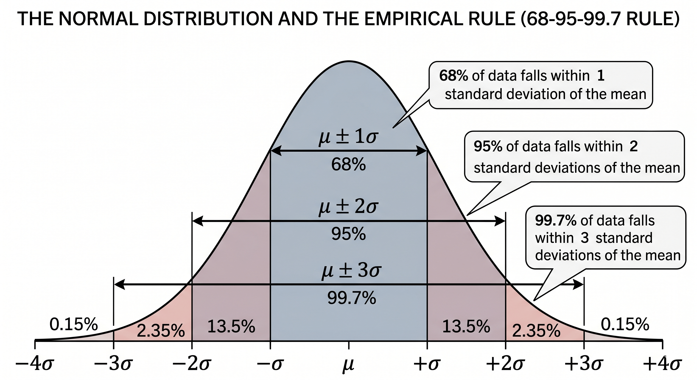
The 68–95–99.7 Empirical Rule (Three-Sigma Rule)
The empirical rule (three-sigma rule) states that in any normal distribution, fixed percentages of data always fall within specific multiples of the standard deviation from the mean. This predictability is what makes standard deviation so actionable in quality control, grading, and clinical reference ranges.
A value beyond ±3σ occurs fewer than 0.27% of the time — these are your statistical outliers. Six Sigma manufacturing targets ±6σ process control, producing fewer than 3.4 defects per million opportunities. This directly extends the empirical rule to extreme quality tolerances.
Low vs. High Standard Deviation: Real-World Interpretation
The same numerical SD can mean very different things depending on context. A standard deviation of 10 on a 100-point exam (mean 70) is moderate — 68% of students scored between 60 and 80. A standard deviation of 10 on a manufacturing tolerance of 1.00mm (mean 1.00mm) is catastrophic. Always interpret σ relative to the scale and purpose of the measurement.
CV = (σ / μ) × 100%
CV lets you compare variability across datasets with different units or magnitudes. A stock with mean return = 8% and σ = 4% has CV = 50%. A bond with mean return = 3% and σ = 0.5% has CV = 16.7% — far more consistent relative to its return.
What Is the Difference Between Standard Deviation and Variance?
Variance is the average of squared deviations from the mean (σ²); standard deviation is the square root of variance (σ). Standard deviation is in the same units as the data; variance is in squared units, making it harder to interpret directly.
Table: Standard Deviation vs. Variance — Direct Comparison
| Property | Standard Deviation | Variance |
|---|---|---|
| Formula | √(∑(x−μ)² / N) | ∑(x−μ)² / N |
| Symbol | σ (population), s (sample) | σ² (population), s² (sample) |
| Units | Same as original data (e.g., cm, $, points) | Squared units (cm², $², points²) |
| Interpretability | Easy — directly comparable to data values | Hard — squared units are not intuitive |
| Mathematical use | Reporting, charts, empirical rule | ANOVA, regression, theoretical proofs |
| Relationship | s = √(s²) | s² = s² |
What Is the Difference Between Standard Deviation and Standard Error?
Standard deviation (s) measures the spread of individual values within a dataset. Standard error (SE = s/√n) measures the precision of the sample mean as an estimate of the population mean. They answer different questions — use standard deviation for descriptive statistics; use standard error for inferential statistics and confidence intervals.
Example: If s = 9.072 and n = 25, then SE = 9.072 / √25 = 9.072 / 5 = 1.814.
This means: with a sample of 25, the sample mean is expected to vary by about ±1.81 points from the true population mean.
A common error: reporting SE instead of SD when describing data spread makes your data look more consistent than it is. SD describes how individual measurements vary; SE describes how repeatable your sample mean would be if you re-sampled. For an authoritative distinction, see Penn State’s STAT 500 Applied Statistics course, which covers this distinction in detail as part of sampling distributions.
Standard Deviation in Excel, Python, and R
Every major data tool has a built-in standard deviation function. The key difference to watch is whether the function uses N (population) or n−1 (sample). Getting this wrong silently introduces a bias into your analysis.
Microsoft Excel
=STDEV.S(A1:A10)    // Sample SD — divides by n-1   ✓ USE THIS for most research
=STDEV.P(A1:A10)    // Population SD — divides by N  ✓ USE when you have all data
=VAR.S(A1:A10)      // Sample Variance (s²)
=VAR.P(A1:A10)      // Population Variance (σ²)
=AVERAGE(A1:A10)    // Mean (needed before computing SD manually)

// Legacy functions (still work but use the newer .S/.P versions):
=STDEV()    // Same as STDEV.S
=STDEVP()   // Same as STDEV.P
Python (NumPy / SciPy)
import numpy as np

data = [72, 85, 90, 68, 77]

# Sample standard deviation (ddof=1 = Bessel's correction, n-1)
s = np.std(data, ddof=1)
print(f"Sample SD: {s:.4f}")          # 9.0720

# Population standard deviation (ddof=0 = divide by N)
sigma = np.std(data, ddof=0)
print(f"Population SD: {sigma:.4f}")  # 8.1111

# Sample variance
var = np.var(data, ddof=1)
print(f"Sample Variance: {var:.4f}")  # 82.30

# Mean
mean = np.mean(data)
print(f"Mean: {mean:.1f}")            # 78.4

# GOTCHA: np.std() uses ddof=0 by default (population).
# Always pass ddof=1 for sample standard deviation.
R Language
data <- c(72, 85, 90, 68, 77)

# Sample standard deviation (R uses n-1 by default — same as Bessel's correction)
sd(data)          # 9.072012

# Sample variance
var(data)         # 82.3

# Mean
mean(data)        # 78.4

# Population standard deviation — R has no built-in; compute manually:
pop_sd <- sqrt(sum((data - mean(data))^2) / length(data))
pop_sd            # 8.111164

# Summary statistics
summary(data)     # Min, Q1, Median, Mean, Q3, Max
Real-World Applications of Standard Deviation
Standard deviation is not just a classroom concept. Three industries depend on it as a core operational metric.
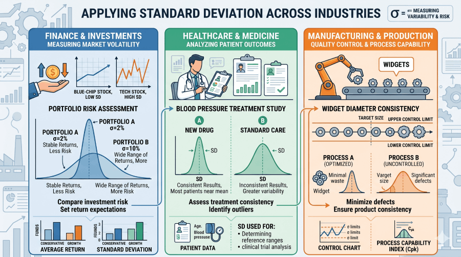
Finance: Asset Volatility and the Sharpe Ratio
In finance, standard deviation of a stock’s returns is the standard measure of investment risk — often called volatility. A stock with annualized σ = 5% is considered low-risk; one with σ = 40% is high-risk. The Sharpe ratio (S = (R𝑝 − R𝑓) / σ𝑝), developed by Nobel laureate William F. Sharpe, divides excess return by the portfolio’s standard deviation to measure risk-adjusted performance. A higher Sharpe ratio indicates better return per unit of risk taken. See Statistics and Probability for related concepts in probability distributions.
Healthcare: Clinical Reference Ranges
Clinical laboratories define "normal" blood test ranges using ±2 standard deviations from the mean value in a healthy reference population. Because 95.45% of healthy values fall within μ±2σ, any patient result outside that range flags as clinically abnormal. For example, a fasting glucose test might have μ = 90 mg/dL and σ = 8 mg/dL, making the normal range 74–106 mg/dL. Standard deviation here directly defines what “healthy” means in measurable terms. For further reading on how population data informs clinical cutoffs, see the WHO guidelines on reference intervals and decision limits.
Manufacturing: Six Sigma Quality Control
Six Sigma (6σ) is a quality management methodology that defines a near-perfect process as one producing fewer than 3.4 defects per million opportunities — corresponding to the area beyond ±6σ from the process mean. Developed at Motorola and later adopted by General Electric, Six Sigma treats standard deviation as the central engineering metric. A process where all output falls within ±3σ of the specification target (a common initial standard) still produces 2,700 defects per million. Tightening to ±6σ reduces that to 3.4. This extends the empirical rule to an extreme tolerance engineering context. See also Study Design for how variance control applies to experimental methods.
Standard Deviation: Complete Formula and Entity Reference
The table below covers every key formula and concept connected to standard deviation. It is structured for quick reference by students, practitioners, and AI retrieval systems.
Table: Standard Deviation Formula Glossary
| Concept | Formula | Plain Explanation | Primary Use |
|---|---|---|---|
| Population SD | σ = √(∑(x−μ)² / N) | Spread of all values in a complete population around the population mean | Complete datasets: census, full class records, entire production batch |
| Sample SD | s = √(∑(x−x̄)² / (n−1)) | Spread of a sample, corrected to estimate the population SD unbiasedly | Research samples, surveys, experiments — the most common case |
| Population Variance | σ² = ∑(x−μ)² / N | Average squared distance from the mean; SD squared | ANOVA, regression, theoretical derivations |
| Sample Variance | s² = ∑(x−x̄)² / (n−1) | Sample version of variance; unbiased estimator of σ² | F-tests, variance decomposition in ANOVA |
| Standard Error of Mean | SE = s / √n | How precisely the sample mean estimates the true population mean | Confidence intervals: x̄ ± z* × (s/√n) |
| Z-Score | z = (x − μ) / σ | How many standard deviations x is from the mean | Comparing values across distributions; probability lookups |
| Coefficient of Variation | CV = (σ / μ) × 100% | SD as a percentage of the mean; scale-free measure of variability | Comparing variability across datasets with different units |
| Empirical Rule | μ±1σ = 68.27%, μ±2σ = 95.45%, μ±3σ = 99.73% | Fixed proportions of normally distributed data within each σ band | Quality control (Six Sigma); grading curves; clinical reference ranges |
| Confidence Interval | CI = x̄ ± z* × (s / √n) | Range likely to contain the true population mean at a given confidence level | Reporting research findings; hypothesis testing |
| Bessel’s Correction | Denominator: (n−1) instead of n | Corrects the downward bias in sample variance as an estimator of σ² | Any computation of sample variance or sample SD |
Standard Deviation and Simple Linear Regression
Standard deviation is a foundational building block of simple linear regression: the slope of the regression line equals the correlation coefficient multiplied by the ratio of the standard deviations of Y and X. Understanding SD is therefore a prerequisite for regression analysis.
b₁ = r × (sₐ / sₓ)
Where r = Pearson correlation, sₐ = standard deviation of Y, sₓ = standard deviation of X.
This shows that a variable with higher variability (larger SD) relative to the other has proportionally more influence on the slope.
See the full treatment in the Simple Linear Regression guide on Statistics Fundamentals.
Related Topics on Statistics Fundamentals
Standard deviation connects to nearly every area of statistics. These pages build the full picture.
Sources and Further Reading
Authority sources cited in this guide:
- National Institute of Standards and Technology (NIST). Engineering Statistics Handbook — Measures of Scale. itl.nist.gov
- MIT OpenCourseWare. 18.650 Statistics for Applications, Fall 2016. ocw.mit.edu
- Penn State STAT 500. Applied Statistics. online.stat.psu.edu
- UC Berkeley Department of Statistics. statistics.berkeley.edu
- World Health Organization. Reference Intervals and Decision Limits. who.int
- Wikipedia contributors. Standard deviation. en.wikipedia.org
- Wackerly, Mendenhall & Scheaffer. Mathematical Statistics with Applications, 7th ed. Cengage Learning, 2008.
Frequently Asked Questions
Standard deviation measures how spread out the values in a dataset are around their mean. It is the square root of variance, calculated as σ = √(∑(x−μ)²/N) for a population and s = √(∑(x−x̄)²/(n−1)) for a sample. A low standard deviation means data clusters tightly near the mean; a high one means values are widely scattered.
Population standard deviation (σ) uses all data points and divides by N. Sample standard deviation (s) uses a subset and divides by n−1, applying Bessel’s correction to avoid underestimating spread. Use σ when you have complete data; use s when working from a sample to estimate the whole population. In Excel: STDEV.P() for population; STDEV.S() for sample.
A low standard deviation means data points cluster tightly around the mean, indicating consistency. A high standard deviation means values are spread widely, indicating variability. For example, σ = 2 on a 100-point test means scores are very consistent; σ = 20 means scores varied dramatically across students. Context matters: always interpret σ relative to the scale of your data — a standard deviation of 10 means very different things for exam scores versus nanometer-scale manufacturing tolerances.
Bessel’s correction is the use of n−1 instead of n in the denominator of the sample variance formula. Named after Friedrich Bessel (1784–1846), this correction ensures the sample variance is an unbiased estimator of the population variance. Without it, sample variance would systematically underestimate the true population spread because sample data points tend to cluster closer to the sample mean than to the true population mean. Every major statistics software applies this correction by default when you compute a sample standard deviation.
Variance is the average of squared deviations from the mean (σ²), while standard deviation is the square root of variance (σ = √σ²). Standard deviation is expressed in the same units as the original data — dollars, points, centimeters — making it easy to interpret. Variance is in squared units, which are difficult to interpret directly but are essential for mathematical proofs, ANOVA, and regression analysis. For everyday reporting, use standard deviation; for mathematical operations, use variance.
Standard deviation (s) measures the spread of individual data points within a dataset. Standard error (SE = s/√n) measures the precision of the sample mean as an estimate of the population mean. Use standard deviation when describing the variability of your data; use standard error when making inferences about the population mean or constructing confidence intervals. Standard error shrinks as sample size increases — more data means a more precise mean estimate — while standard deviation stays relatively stable regardless of sample size.
In Excel, use =STDEV.S(range) for sample standard deviation (divides by n−1, correct for most research) or =STDEV.P(range) for population standard deviation (divides by N). For example, =STDEV.S(A1:A10) returns the sample standard deviation of the ten values in cells A1 through A10. For variance, use =VAR.S() or =VAR.P() respectively.
For the dataset {1, 2, 3, 4, 5}: Mean = 3. Squared deviations: (1−3)²=4, (2−3)²=1, (3−3)²=0, (4−3)²=1, (5−3)²=4. Sum = 10. Population variance = 10/5 = 2, so population SD = √2 ≈ 1.414. Sample variance = 10/4 = 2.5, so sample SD = √2.5 ≈ 1.581. Enter these values into the calculator above to verify.