You open a statistics textbook and hit the word heteroscedasticity. You read a data science paper and see Bayesian posterior. You see a confidence interval in a news story and wonder what it actually means. Every one of those moments is a vocabulary problem — and vocabulary problems have fast solutions. This glossary gives you exact, formula-complete definitions for every essential statistics term, written so they hold up whether you're preparing for an exam, running a research project, or wrangling data in Python.
The glossary covers six categories: descriptive statistics, probability and distributions, inferential statistics, sampling, correlation and regression, and statistical tests. Each entry follows the same structure: definition, formula (where applicable), one concrete example, and links to the full topic guides on Statistics Fundamentals.
What This Glossary Covers
✓ 150+ terms across 6 core statistical categories
✓ Every definition written in plain English — no jargon without explanation
✓ Exact formulas with variable definitions for every quantitative term
✓ Concrete real-world examples for the 30 most-tested terms
✓ Statistical tests reference table with use cases, assumptions, and outputs
✓ Interactive search and filter by category
What Is a Statistics Glossary? (And How to Use This Guide)
Definition — Statistics Glossary
A statistics glossary is a curated reference of standardized definitions for the concepts, measures, tests, and methods used in statistical analysis. Each entry maps a term to its precise mathematical meaning, formula, and real-world application — giving students and practitioners a single authoritative source for statistical vocabulary.
Statistics has a vocabulary problem. The same concept often goes by two or three different names — standard score, z-score, and z-value all refer to the same thing. Some terms sound identical but mean different things — standard deviation and standard error are related but distinct. And a handful of terms, like significance, mean something quite specific in statistics that differs from everyday usage.
This glossary resolves that. Each term appears once, under its most commonly used name, with cross-references to synonyms. Use the search bar below to jump directly to a term, or browse by letter using the alphabet navigator. Click any term card to expand the full definition, formula, and example.
For deeper coverage of each topic — with step-by-step worked examples, interactive calculators, and Python/R code — follow the linked topic guides throughout the glossary. Every formula in this reference has been verified against the NIST/SEMATECH Engineering Statistics Handbook and standard university-level textbooks including OpenIntro Statistics.
150+
Terms Defined
6
Categories
30+
Formulas Included
25+
Worked Examples
Search the Glossary
Showing all 150+ terms
Core Descriptive Statistics Terms
Descriptive statistics summarize and describe the characteristics of a dataset. Unlike inferential statistics, descriptive methods do not attempt to draw conclusions beyond the data collected. They answer: "What does this data look like?" rather than "What does this data tell us about a larger population?" According to Khan Academy's statistics curriculum, descriptive statistics form the essential foundation for all further statistical reasoning.
A
Alternative hypothesis (H₁) is the statement that contradicts the null hypothesis — it proposes that a real effect, difference, or relationship exists. It is what the researcher typically hopes to demonstrate. H₁ is accepted when the p-value falls below the chosen significance level (α), causing rejection of H₀.
Example H₀: A new drug has no effect on blood pressure. H₁: The drug reduces blood pressure. If the study produces p = 0.02 and α = 0.05, H₀ is rejected in favor of H₁.
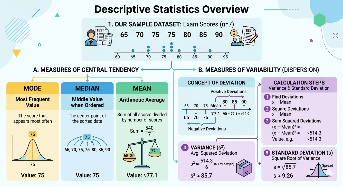
The arithmetic mean is the most common measure of central tendency. It equals the sum of all data values divided by the number of values. The population mean uses symbol μ (mu); the sample mean uses x̄ (x-bar). The mean is sensitive to outliers — a single extreme value can pull it far from the data's center, making it less reliable for skewed distributions.
μ = Σxᵢ / N | x̄ = Σxᵢ / n
Example Test scores: 70, 75, 80, 85, 90. Mean = (70+75+80+85+90) / 5 = 400 / 5 = 80. Each score deviates from 80 by different amounts — standard deviation measures that spread.
Average absolute deviation measures spread by computing the mean of the absolute (non-negative) distances between each data point and the dataset's mean. Unlike variance, it does not square deviations, so it remains in the original units and is less sensitive to outliers than standard deviation. It sees use in finance and forecasting accuracy (MAE — mean absolute error).
Bayes' theorem describes how to update the probability of a hypothesis (the prior probability) given new evidence. The result — the posterior probability — reflects both prior belief and the likelihood of the observed evidence. It underpins Bayesian statistics, spam filtering, medical diagnosis, and machine learning classification. Named after Reverend Thomas Bayes (1763).
P(A|B) = [P(B|A) · P(A)] / P(B)
Example A medical test for a disease has 99% sensitivity and 99% specificity. The disease affects 1% of the population. If a person tests positive, P(disease | positive) ≈ 50% — not 99%. Bayes' theorem accounts for the low base rate, which raw test accuracy ignores. Source: NIH — Understanding Bayes' Theorem.
The binomial distribution models the number of successes in a fixed number of independent trials, each with the same probability of success (p). It applies when: there are exactly two outcomes (success/failure), trials are independent, n is fixed, and p is constant. The mean of a binomial distribution equals np; the variance equals np(1−p).
A box plot displays the five-number summary of a dataset: minimum, Q1, median (Q2), Q3, and maximum. The box spans from Q1 to Q3 (the interquartile range). Whiskers extend to the farthest non-outlier values. Data points beyond 1.5 × IQR from the box edges are plotted individually as potential outliers. Box plots make skewness and outliers immediately visible.
Example Exam scores with Q1=65, Median=75, Q3=85 produce a box from 65–85. Any score below 65 − 1.5(20) = 35 or above 85 + 1.5(20) = 115 appears as an outlier point.
The Central Limit Theorem (CLT) states that the distribution of sample means approaches a normal distribution as the sample size increases, regardless of the population's underlying distribution. This applies when n ≥ 30 (a common rule of thumb). The sampling distribution of the mean has mean μ and standard deviation σ/√n (the standard error). The CLT is why normal-distribution methods work across so many real-world problems — it is the theoretical backbone of most inferential statistics.
x̄ ~ N(μ, σ²/n) as n → ∞
Example A population of incomes is heavily right-skewed. But if you take 1,000 random samples of n=50 and compute each sample mean, those means form an approximately normal bell curve centered on the true population mean. This is the CLT at work. Source: Yale Statistics — Central Limit Theorem.
A confidence interval is a range of values, calculated from sample data, that is likely to contain the true population parameter with a specified probability (confidence level). A 95% CI does not mean there is a 95% chance the parameter lies within this specific interval — it means that 95% of all such intervals constructed from repeated sampling would contain the true parameter. Common confidence levels: 90% (z*=1.645), 95% (z*=1.96), 99% (z*=2.576).
CI = x̄ ± z* · (σ/√n)
Example A poll of 1,000 voters finds 52% support a candidate. With a 95% CI: 52% ± 1.96 · √(0.52·0.48/1000) ≈ 52% ± 3.1%. The CI is [48.9%, 55.1%] — meaning the true support is likely between 48.9% and 55.1%.
Pearson's correlation coefficient (r) measures the strength and direction of the linear relationship between two continuous variables. It ranges from −1 (perfect negative linear relationship) to +1 (perfect positive linear relationship), with 0 indicating no linear relationship. Correlation does not imply causation — two variables can correlate strongly due to a third confounding variable.
r = Σ[(xᵢ−x̄)(yᵢ−ȳ)] / √[Σ(xᵢ−x̄)²·Σ(yᵢ−ȳ)²]
Example Height and weight across 100 adults: r = 0.68 (moderate positive correlation). Ice cream sales and drowning deaths: r ≈ 0.85 — but both are caused by hot weather (a confounder), not by each other.
The coefficient of variation (CV) expresses the standard deviation as a percentage of the mean. It measures relative variability, making it useful for comparing spread across datasets with different units or means. A lower CV indicates more consistency relative to the average; a higher CV indicates more relative dispersion.
CV = (σ / μ) × 100%
Example Dataset A: mean=100, SD=10 → CV=10%. Dataset B: mean=10, SD=2 → CV=20%. Although dataset A has a larger absolute SD, dataset B has more relative variability.
D
Degrees of freedom (df) refers to the number of independent values in a dataset that can vary freely when computing a statistic. When estimating the sample mean from a dataset of n values, one degree of freedom is "used up" constraining the sum — leaving n−1 free. This is why sample variance divides by n−1 (Bessel's correction) rather than n. The t-distribution's shape depends on df — more df means it approaches the normal distribution.
df = n − 1 (one-sample t-test)
Example With 10 observations and one estimated mean, df = 9. Looking up a critical t-value at α=0.05 (two-tailed) with df=9 gives t* = 2.262 — notably higher than the normal distribution's z* = 1.96, reflecting uncertainty from the small sample.
Descriptive statistics encompasses methods for summarizing, organizing, and displaying the main features of a dataset without drawing conclusions beyond the data. The two main types are measures of central tendency (mean, median, mode) and measures of variability (range, variance, standard deviation, IQR). Descriptive statistics answer "What does this data look like?" — the foundation before any inferential analysis begins.
Example A school reports exam results: mean = 74, median = 76, SD = 12, range = 45–100. These five numbers describe the entire dataset without requiring inspection of 300 individual scores.
A discrete variable takes countable, separate values — typically whole numbers. A continuous variable can take any value within a range, including decimals and fractions. The distinction determines which probability distribution applies: discrete variables use the binomial, Poisson, or geometric distributions; continuous variables use the normal, exponential, or uniform distributions.
Example Number of customers entering a store (0, 1, 2, 3…) is discrete. The time between customer arrivals (0.0–∞ seconds) is continuous. You can have exactly 3 customers but not 3.5 customers.
Effect size measures the practical magnitude of a finding, independent of sample size. Statistical significance (p-value) answers "Is this effect real?" — effect size answers "How large is it?" Cohen's d is the most common effect size for comparing two means: d = 0.2 is small, d = 0.5 is medium, d = 0.8 is large. A study can be statistically significant with a tiny effect size if the sample is very large.
d = (μ₁ − μ₂) / σ_pooled
Example A new teaching method raises test scores from 70 to 75 (SD=10). d = (75−70)/10 = 0.5 — a medium effect. The improvement is real and meaningful, not just statistically detectable noise.
Expected value E[X] is the long-run average value of a random variable over many repetitions of an experiment. For a discrete random variable, it equals the sum of each possible value multiplied by its probability. For continuous random variables, it equals the integral of x·f(x). The expected value is the population mean — it need not be a value the variable can actually take.
E[X] = Σ xᵢ · P(xᵢ)
Example A fair six-sided die: E[X] = (1+2+3+4+5+6)/6 = 3.5. You can never roll a 3.5, but over thousands of rolls, the average converges to 3.5.
F
The five-number summary describes a dataset using five values: the minimum, the first quartile (Q1, 25th percentile), the median (Q2, 50th percentile), the third quartile (Q3, 75th percentile), and the maximum. Together these capture the center, spread, and overall range of the data. Box plots visualize this summary directly.
The F-statistic is the ratio of variance between groups to variance within groups. A large F-value suggests that at least one group mean differs significantly from the others. The F-test is the foundation of ANOVA (Analysis of Variance). It also appears in regression analysis to test whether the model as a whole is statistically significant. Critical F-values depend on two degrees of freedom: numerator (k−1) and denominator (N−k).
F = (MS_between) / (MS_within)
Example Comparing exam scores across three teaching methods. F = 8.3, p = 0.001 → reject H₀ that all three methods produce equal means. At least one method differs significantly. Use the F-table to find critical values.
Hypothesis testing is a formal procedure for using data to evaluate competing claims about a population. It begins with a null hypothesis (H₀, no effect) and an alternative hypothesis (H₁, some effect). A test statistic is computed from sample data and compared to a critical value or converted to a p-value. If p < α (the significance level, typically 0.05), H₀ is rejected.
The 5-Step Framework
State H₀ and H₁
Choose significance level α (typically 0.05)
Select and compute the appropriate test statistic
Find the p-value (or compare to critical value)
Reject or fail to reject H₀
Related: Hypothesis Testing Guide, P-Value, Type I Error, Type II Error, Statistical Significance
I
The interquartile range (IQR) measures the spread of the middle 50% of data by subtracting the first quartile (Q1, 25th percentile) from the third quartile (Q3, 75th percentile). Because it ignores the lowest and highest 25% of values, the IQR is resistant to outliers — making it a more reliable measure of spread than range or standard deviation when data is skewed. Outlier detection often uses 1.5 × IQR as a threshold.
IQR = Q3 − Q1
Example Income data: Q1=$40,000, Q3=$80,000. IQR = $40,000. An outlier threshold: values below Q1 − 1.5(40,000) = −$20,000 or above Q3 + 1.5(40,000) = $140,000 are flagged as potential outliers.
Related: Quartiles, Box Plot, Outliers, Range, Standard Deviation
Inferential statistics uses data from a sample to draw conclusions about the population it was drawn from. Unlike descriptive statistics (which only describe the data at hand), inferential methods account for uncertainty through probability — using tools like confidence intervals, hypothesis tests, and regression models. The validity of inferential conclusions depends on how well the sample represents the population.
Example A poll of 1,200 voters (a sample) is used to estimate the voting preferences of 150 million eligible voters (the population). Every presidential election poll relies on inferential statistics.
Kurtosis measures the "tailedness" of a probability distribution — how much probability mass sits in the tails versus the center, compared to a normal distribution. A normal distribution has kurtosis = 3 (excess kurtosis = 0). Leptokurtic distributions (excess kurtosis > 0) have heavy tails and more outliers. Platykurtic distributions (excess kurtosis < 0) have thin tails and fewer outliers. Mesokurtic distributions match the normal distribution.
κ = [Σ(xᵢ−μ)⁴/n] / σ⁴ (excess: κ − 3)
Example Financial return distributions are typically leptokurtic — extreme gains or losses happen more often than a normal distribution would predict. This is why standard financial risk models underestimate "black swan" events.
L
The Law of Large Numbers states that as the number of trials or observations increases, the sample mean converges to the population mean (μ). The weak LLN (Chebyshev) guarantees convergence in probability; the strong LLN (Borel) guarantees almost sure convergence. The LLN justifies why large samples are more reliable than small ones and underpins the logic of insurance, casinos, and epidemiology.
Example Rolling a fair die 10 times might yield an average of 2.8 or 4.1 — far from the expected 3.5. Roll it 10,000 times and the average will be very close to 3.5. The LLN guarantees this convergence.
Simple linear regression models the relationship between one predictor variable (X) and one outcome variable (Y) using a straight line. The slope (β₁) quantifies how much Y changes for each one-unit increase in X. The intercept (β₀) gives the predicted Y when X = 0. The line is fit using ordinary least squares (OLS) — minimizing the sum of squared residuals (vertical distances from data points to the line).
ŷ = β₀ + β₁x | β₁ = r · (Sᵧ / Sₓ)
Example Predicting salary (Y) from years of experience (X). If β₀ = $35,000 and β₁ = $5,000, the model predicts a starting salary of $35,000 and $5,000 added per year of experience.
The margin of error quantifies the uncertainty in a sample-based estimate. It represents the half-width of a confidence interval — the maximum likely distance between the sample statistic and the true population parameter at a given confidence level. Margin of error decreases as sample size increases and as the confidence level decreases.
MoE = z* · (σ/√n)
Example A poll reports "48% support, ±3 percentage points." The ±3% is the margin of error at 95% confidence — meaning the true population support is estimated to be between 45% and 51%.
See Arithmetic Mean above. Three other mean types exist: Geometric mean = (x₁·x₂·…·xₙ)^(1/n), used for growth rates. Harmonic mean = n / Σ(1/xᵢ), used for rates. Weighted mean = Σ(wᵢxᵢ) / Σwᵢ, used when observations contribute unequally (e.g., GPA calculation).
The median is the middle value of a dataset when arranged in ascending order. For an odd number of values, it is the central value. For an even number, it is the mean of the two middle values. The median is resistant to outliers — making it the preferred central tendency measure for skewed distributions (e.g., income, housing prices) where the mean is pulled toward extreme values.
Example Odd dataset: 10, 20, 30, 40, 50 → Median = 30. Even dataset: 10, 20, 30, 40 → Median = (20+30)/2 = 25. If we add an outlier (10, 20, 30, 40, 1000): Mean = 220, Median = 30. The median barely moves; the mean jumps dramatically.
The mode is the value that occurs most frequently in a dataset. A dataset can have one mode (unimodal), two modes (bimodal), multiple modes (multimodal), or no mode if all values are equally frequent. The mode is the only central tendency measure that applies to categorical (nominal) data — you can find the most common eye color but not the "mean" or "median" eye color.
Example Shoe sizes sold: 7, 8, 8, 9, 9, 9, 10, 10. Mode = 9 (appears 3 times). A shoe store stocks more size 9s based on this. For continuous data measured in bins (e.g., histogram), the mode is the bin with the highest frequency.
Mutually exclusive events cannot both occur at the same time — if one happens, the other cannot. P(A and B) = 0 for mutually exclusive events. Independent events have no influence on each other — knowing one occurred gives no information about the other. P(A and B) = P(A) × P(B) for independent events. Mutually exclusive events are never independent (unless one has probability 0) because knowing one occurred tells you the other did not.
Example Rolling a 3 and rolling a 5 on one die roll: mutually exclusive. Rolling two different dice: each roll is independent — the result of one die does not affect the other.
N
The normal distribution (also called Gaussian distribution or bell curve) is the most important probability distribution in statistics. It is symmetric, unimodal, and bell-shaped, fully described by its mean (μ) and standard deviation (σ). About 68% of data falls within ±1σ, 95% within ±2σ, and 99.7% within ±3σ (the 68-95-99.7 empirical rule). The standard normal distribution has μ=0 and σ=1 — all z-scores map onto it.
f(x) = (1/σ√2π) · e^[−(x−μ)²/2σ²]
Example Human heights, IQ scores, blood pressure readings, and measurement errors all approximate normal distributions. This is why the normal distribution is ubiquitous — the Central Limit Theorem guarantees that sample means follow it regardless of the underlying distribution.
The null hypothesis (H₀) is the default assumption that there is no effect, no difference, or no relationship between variables. Hypothesis testing attempts to disprove H₀ using evidence from sample data. "Failing to reject H₀" is not the same as proving H₀ true — it means the data does not provide sufficient evidence against it. The burden of proof rests on demonstrating that H₀ is implausible, not on proving H₀ false.
Example Testing whether a coin is fair: H₀: P(heads) = 0.5. You flip the coin 100 times and get 72 heads. p-value ≈ 0.00008 — far below 0.05. You reject H₀ and conclude the coin is likely biased.
Related: Hypothesis Testing, Alternative Hypothesis, P-Value, Type I Error
O
An outlier is a data point that lies far from the bulk of the distribution. Two common detection methods: the z-score method (flag values with |z| > 3 — affects <0.3% of normally distributed data) and the IQR method (flag values below Q1 − 1.5·IQR or above Q3 + 1.5·IQR). Outliers may reflect genuine extreme values, measurement errors, or data entry mistakes. Removing them arbitrarily without investigation is bad practice.
Example Household income dataset: $40k, $50k, $55k, $60k, $2.3M. The $2.3M observation is an outlier that raises the mean dramatically while the median remains near $55k — illustrating why the median better represents typical income.
P
A parameter is a numerical characteristic of a population (e.g., population mean μ, population proportion π, population standard deviation σ). A statistic is a numerical characteristic computed from a sample (e.g., sample mean x̄, sample proportion p̂, sample standard deviation s). Statistics are used to estimate unknown parameters. Parameters use Greek letters; statistics use Latin letters.
Example The exact average height of all 8 billion humans on Earth is a parameter (μ) — unknowable without measuring everyone. The average height of 10,000 randomly selected humans (x̄) is a statistic used to estimate μ.
A p-value is the probability of obtaining results at least as extreme as the observed data, assuming the null hypothesis is true. It does not measure the probability that H₀ is true — a common misconception. A small p-value means the data is unlikely under H₀, providing evidence against it. By convention, p < 0.05 is used as the significance threshold, though this threshold is arbitrary and context-dependent. The American Statistical Association's 2016 statement cautions against mechanical p-value cutoffs. Source: ASA P-Value Statement.
Example A clinical trial of a new drug produces p = 0.02. This means: if the drug truly had no effect (H₀), there is only a 2% chance of observing results this extreme. Since 2% < 5% threshold, H₀ is rejected — evidence supports a real drug effect.
Related: Hypothesis Testing, Statistical Significance, Type I Error, Null Hypothesis
The population is the complete set of individuals, objects, or events that a study aims to describe or make inferences about. The sample is the subset of the population that is actually observed and measured. Because studying entire populations is often impractical or impossible, inferential statistics uses sample data to estimate population characteristics. A representative sample is critical — a biased sample yields systematically wrong estimates.
Example Studying the average sleep duration of US adults (population: ~260 million adults). Researchers measure sleep in a sample of 3,000 randomly selected adults and use that sample to estimate the population average.
Probability is a numerical measure of the likelihood that a specific event will occur, ranging from 0 (impossible) to 1 (certain). The classical definition assumes equally likely outcomes. The frequentist definition defines probability as the long-run relative frequency of an event. The Bayesian definition treats probability as a degree of belief updated with new evidence. All three definitions obey the same axioms (Kolmogorov, 1933).
P(A) = Number of favorable outcomes / Total number of possible outcomes
Example Rolling a fair six-sided die: P(rolling a 4) = 1/6 ≈ 0.167. P(rolling an even number) = 3/6 = 0.5. P(rolling a 7) = 0/6 = 0 (impossible).
A probability distribution specifies all possible values a random variable can take and their associated probabilities. For discrete variables: the Probability Mass Function (PMF) gives exact probabilities for each value. For continuous variables: the Probability Density Function (PDF) gives probabilities over intervals, and the Cumulative Distribution Function (CDF) gives P(X ≤ x) for any x. Common distributions include normal, binomial, Poisson, exponential, and uniform.
Example Standard normal distribution: the PDF gives the bell curve shape; the CDF gives the probability that Z falls at or below any z-value — which is exactly what the z-table reports.
Related: Normal Distribution, Binomial Distribution, Random Variables
R
The range is the simplest measure of spread: the difference between the largest and smallest values in a dataset. It captures the full extent of the data but is highly sensitive to outliers — a single extreme value drastically changes the range. For skewed data or data with outliers, the IQR is a more robust spread measure.
Range = Maximum − Minimum
Example Test scores: 62, 70, 75, 80, 88, 95. Range = 95 − 62 = 33. If one student scores 20 (outlier): Range = 95 − 20 = 75 — the range doubled due to one unusual score.
R-squared (R²) measures the proportion of variance in the dependent variable explained by the regression model. It ranges from 0 to 1: R² = 0 means the model explains nothing; R² = 1 means the model explains all variation (perfect fit). R² = 0.75 means 75% of the variance in Y is accounted for by the predictor(s). Higher R² does not guarantee a good model — it can always be inflated by adding more predictors (use Adjusted R² instead for multiple regression).
R² = 1 − (SS_residual / SS_total)
Example Salary predicted from years of experience: R² = 0.65. Experience explains 65% of salary variance. The remaining 35% depends on other factors (education, industry, location) not in the model.
A residual is the difference between an observed value and the value predicted by the regression model. Residuals measure how far the model's predictions deviate from the actual data. Ordinary least squares (OLS) regression minimizes the sum of squared residuals. Residual analysis — checking for patterns, normality, and constant variance (homoscedasticity) — is a critical step in validating regression assumptions.
eᵢ = yᵢ − ŷᵢ
Example A salary model predicts $65,000 for a candidate who actually earns $72,000. Residual = 72,000 − 65,000 = $7,000 (positive — the model underestimated this observation).
S
Sampling bias occurs when the method of selecting a sample systematically favors certain members of the population over others, producing estimates that do not reflect the population. Common types include: selection bias (non-random selection), survivorship bias (only studying "survivors"), nonresponse bias (certain groups systematically decline to participate), and volunteer bias (self-selected participants differ from the general population).
Example The 1936 Literary Digest presidential poll predicted Landon would beat Roosevelt 57%–43%. The poll sampled telephone owners and car owners — disproportionately wealthy and Republican in 1936. Roosevelt won by a landslide. Classic survivorship bias example: studying only planes that returned from WWII missions to reinforce them — ignoring where shot-down planes were hit.
The sample size (n) is the number of observations in a study. Larger samples produce more precise estimates (smaller margin of error), increase statistical power (ability to detect real effects), and better satisfy the conditions of the Central Limit Theorem. However, larger samples cost more time and money. Power analysis — conducted before data collection — determines the minimum n needed to detect an effect of a given size with specified confidence and power.
Example To achieve a margin of error of ±3% at 95% confidence for a proportion near 50%: n = (1.96²·0.5·0.5) / 0.03² ≈ 1,068 observations required.
Related: Study Design, Margin of Error, Statistical Power, Confidence Interval
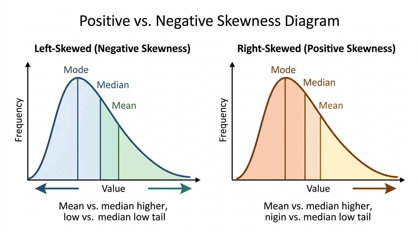
Skewness measures the degree and direction of asymmetry in a distribution. A skewness of 0 indicates a symmetric distribution. Positive (right) skewness means the right tail is longer — the mean is pulled above the median (e.g., income distributions). Negative (left) skewness means the left tail is longer — the mean is pulled below the median (e.g., age at retirement). As a rule: right-skewed → mean > median; left-skewed → mean < median.
γ₁ = [Σ(xᵢ−x̄)³/n] / s³
Example US household income: right-skewed (a few billionaires stretch the right tail). Mean income ≈ $105,000; median ≈ $74,000. The median better represents the "typical" household. The gap between mean and median signals skewness.
The standard error (SE) is the standard deviation of a sampling distribution. For the sample mean, SE = σ/√n — it measures how much sample means vary from sample to sample. As n increases, SE decreases (larger samples give more precise estimates). Do not confuse SE with standard deviation: SD describes spread within a single dataset; SE describes how much a statistic (like the mean) varies across repeated samples.
SE(x̄) = σ / √n | SE(p̂) = √[p(1−p)/n]
Example Population σ = 20, sample n = 100. SE = 20/√100 = 2. If n increases to 400: SE = 20/20 = 1. Quadrupling the sample size halves the standard error.
Related: Sampling Distributions, Confidence Interval, Margin of Error, Central Limit Theorem
Standard deviation measures how spread out data points are around the mean. It is the square root of variance, expressed in the same units as the original data. The population standard deviation (σ) uses N in the denominator; the sample standard deviation (s) uses n−1 (Bessel's correction) to produce an unbiased estimate of the population σ. A small SD means data clusters tightly near the mean; a large SD means data spreads widely.
σ = √[Σ(xᵢ−μ)²/N] | s = √[Σ(xᵢ−x̄)²/(n−1)]
Example Class A: mean=75, SD=3 (scores tightly clustered). Class B: mean=75, SD=15 (scores spread from ~45 to ~100). Same mean — very different distributions. The SD captures what the mean cannot.
Related: Descriptive Statistics, Variance, Z-Score, Normal Distribution, Coefficient of Variation
A result is statistically significant when the p-value falls below the pre-specified significance level α (alpha), typically 0.05. This indicates that the observed result would occur fewer than 5% of the time if H₀ were true — providing evidence against H₀. Statistical significance is not the same as practical significance (effect size). With very large samples, trivially small differences become statistically significant even when they are meaningless in practice.
Example A website A/B test with 1 million users finds that button color change increases click-through by 0.01%. p < 0.001 (statistically significant). But a 0.01% increase is practically meaningless for most businesses. Statistical significance ≠ practical importance.
Related: P-Value, Effect Size, Statistical Power, Type I Error
T
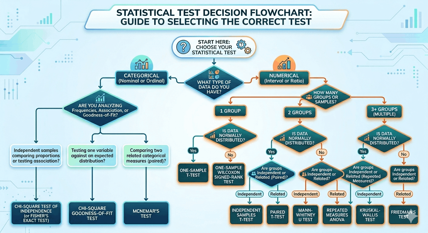
The t-test compares one or two sample means when the population standard deviation is unknown. Three main types: One-sample t-test (compares a sample mean to a known value), Independent two-sample t-test (compares means of two unrelated groups), Paired t-test (compares means from the same group measured twice). The test assumes normally distributed data (or n > 30) and uses the t-distribution with df = n−1 (or n₁+n₂−2 for two samples).
t = (x̄ − μ₀) / (s/√n)
Example Testing whether a class's mean score (x̄=78, s=10, n=25) differs from the national average (μ₀=75). t = (78−75)/(10/5) = 1.5. With df=24, p ≈ 0.147 — not significant at α=0.05. No evidence the class differs from the national average.
A Type I error occurs when the null hypothesis is true but you reject it — a false positive. The probability of a Type I error equals α (the significance level). Setting α = 0.05 means you accept a 5% chance of incorrectly rejecting a true H₀. In medical testing: declaring an ineffective drug effective. In quality control: stopping a production line when nothing is wrong. Reducing α reduces Type I errors but increases Type II errors.
P(Type I Error) = α
Example Null hypothesis: defendant is innocent. Type I error: convicting an innocent person. The criminal justice system sets a very high bar ("beyond reasonable doubt") to minimize Type I errors — at the cost of more Type II errors (acquitting guilty parties).
Related: Type II Error, P-Value, Statistical Significance, Power
A Type II error occurs when the null hypothesis is false but you fail to reject it — a false negative. Its probability is denoted β. Statistical power = 1 − β, representing the probability of correctly detecting a real effect. Type II errors are reduced by increasing sample size, increasing α, or studying larger effects. In medical testing: declaring an effective drug ineffective.
P(Type II Error) = β | Power = 1 − β
Example Null hypothesis: defendant is innocent. Type II error: acquitting a guilty person. In drug testing: a drug that truly reduces blood pressure by 5mmHg goes undetected because the trial was too small to find a statistically significant difference.
Related: Type I Error, Statistical Power, Effect Size, Sample Size
V
Variance measures the average squared deviation of each data point from the mean. Squaring the deviations ensures positive values (positive and negative deviations don't cancel) and weights larger deviations more heavily. Because variance is in squared units (e.g., dollars²), it is less interpretable than standard deviation (which shares the original units). Population variance (σ²) divides by N; sample variance (s²) divides by n−1.
σ² = Σ(xᵢ − μ)² / N | s² = Σ(xᵢ − x̄)² / (n−1)
Example Dataset: 2, 4, 6, 8, 10. Mean = 6. Squared deviations: 16, 4, 0, 4, 16. Population variance = 40/5 = 8. Sample variance = 40/4 = 10. Standard deviation = √8 ≈ 2.83 (population) or √10 ≈ 3.16 (sample).
Related: Standard Deviation, Mean, Covariance, F-Test, ANOVA
Z
A z-score (also called a standard score or z-value) measures how many standard deviations a data point lies above or below the population mean. A z-score of 0 means the value equals the mean. Positive z-scores sit above the mean; negative z-scores sit below it. Z-scores enable comparison of values from distributions with different scales. The process of converting raw values to z-scores is called standardization.
z = (x − μ) / σ
Example A student scores 85 on an exam (μ=70, σ=10). z = (85−70)/10 = 1.5. The student scored 1.5 standard deviations above the mean — approximately the 93rd percentile. Use the z-score calculator or z-table to convert any z-score to a percentile.
What Is the Difference Between Statistical Tests? (Reference Table)
The right statistical test depends on your data type, the number of groups, and the assumptions your data satisfies. Use this table as a decision guide — then follow the links to the full test guides for worked examples and assumption checks.
The table below contains every key formula in this glossary, organized for quick reference. Each formula is verified against the NIST Engineering Statistics Handbook — the authoritative U.S. government reference for statistical methods.
Term
Formula
Variables
Key Note
Population Mean
μ = Σxᵢ / N
xᵢ = values, N = population size
Sensitive to outliers
Sample Mean
x̄ = Σxᵢ / n
n = sample size
Estimates population μ
Population Variance
σ² = Σ(xᵢ−μ)² / N
μ = population mean
Squared units
Sample Variance
s² = Σ(xᵢ−x̄)² / (n−1)
n−1 = Bessel's correction
Unbiased estimate of σ²
Standard Deviation
σ = √[Σ(xᵢ−μ)²/N]
Square root of variance
Same units as data
Z-Score
z = (x − μ) / σ
x = value, σ = SD
Maps to standard normal
Standard Error
SE = σ / √n
σ = population SD
Decreases as n grows
Confidence Interval
CI = x̄ ± z*(σ/√n)
z* = 1.96 for 95% CI
Width shrinks with larger n
Margin of Error
MoE = z* · (σ/√n)
Half-width of CI
±3% typical in polls
t-Statistic (one-sample)
t = (x̄ − μ₀) / (s/√n)
μ₀ = hypothesized mean
df = n − 1
Pearson's r
r = Σ[(xᵢ−x̄)(yᵢ−ȳ)] / √[Σ(xᵢ−x̄)²·Σ(yᵢ−ȳ)²]
Range: −1 to +1
Linear relationship only
Simple Linear Regression
ŷ = β₀ + β₁x
β₀ = intercept, β₁ = slope
OLS minimizes squared residuals
R-Squared
R² = 1 − (SS_res/SS_tot)
Range: 0 to 1
Proportion of variance explained
IQR
IQR = Q3 − Q1
Q1 = 25th, Q3 = 75th percentile
Robust to outliers
Bayes' Theorem
P(A|B) = P(B|A)·P(A) / P(B)
P(A) = prior, P(B|A) = likelihood
Posterior updates prior with evidence
Binomial PMF
P(X=k) = C(n,k)·pᵏ·(1−p)^(n−k)
n = trials, p = success prob
Mean = np, Variance = np(1−p)
Normal PDF
f(x) = (1/σ√2π)·e^[−(x−μ)²/2σ²]
e = Euler's number ≈ 2.718
68-95-99.7 rule applies
Cohen's d
d = (μ₁−μ₂) / σ_pooled
σ_pooled = pooled SD
0.2=small, 0.5=med, 0.8=large
Chi-Square Statistic
χ² = Σ[(O−E)²/E]
O = observed, E = expected
df = (rows−1)·(cols−1)
Expected Value
E[X] = Σ xᵢ · P(xᵢ)
Discrete random variable
= population mean μ
How Do the Major Probability Distributions Compare?
Each probability distribution has a characteristic shape determined by its parameters. The diagrams below illustrate the three most commonly tested distributions in an introductory statistics course.
Normal Distribution — The 68-95-99.7 Rule (Empirical Rule)
The 68-95-99.7 rule: approximately 68% of data falls within ±1σ, 95% within ±2σ, and 99.7% within ±3σ of the mean in any normal distribution.
The most fundamental statistics glossary terms are: mean (arithmetic average), median (middle value), mode (most frequent value), standard deviation (average spread from the mean), variance (average squared deviation), p-value (probability of results under H₀), confidence interval (range containing the true parameter), and null hypothesis (the default assumption of no effect). These eight terms appear in virtually every branch of applied statistics.
A parameter describes a characteristic of the entire population — for example, the population mean μ or population proportion π. A statistic describes a characteristic of a sample drawn from that population — such as the sample mean x̄ or sample proportion p̂. Parameters are typically unknown and estimated using statistics. Parameters are denoted with Greek letters (μ, σ, π); statistics use Latin letters (x̄, s, p̂).
A p-value is the probability of obtaining results at least as extreme as the observed data, assuming the null hypothesis is true. It does not measure the probability that H₀ is true. A p-value below 0.05 means there is less than a 5% chance of seeing such extreme results by chance alone under H₀ — which is the conventional threshold for declaring a result statistically significant and rejecting H₀. The p-value threshold of 0.05 is arbitrary and should be set before data collection.
Standard deviation measures how spread out data points are around the mean. A small standard deviation means most values cluster tightly near the average. A large standard deviation means values are widely scattered. In practical terms: if exam scores have a mean of 70 and a standard deviation of 5, roughly 68% of students scored between 65 and 75. Standard deviation is expressed in the same units as the original data — unlike variance, which is in squared units.
Descriptive statistics summarize and describe the data you have collected — using measures like mean, median, standard deviation, and range. They answer: "What does this data look like?" Inferential statistics use sample data to draw conclusions or make predictions about a larger population — using techniques like hypothesis testing, confidence intervals, and regression. The key difference: descriptive statistics describe only the data at hand; inferential statistics generalize beyond it, with quantified uncertainty.
The Central Limit Theorem (CLT) states that the distribution of sample means approaches a normal distribution as sample size increases, regardless of the population's underlying distribution. This typically applies when n ≥ 30. The CLT matters because it justifies using normal-distribution methods (z-tests, t-tests, confidence intervals) across many real-world problems where the population itself is not normally distributed. Without the CLT, most inferential statistics would require knowing the population's exact distribution shape.
The most critical statistics terms for data science are: mean, variance, standard deviation (feature characterization), normal distribution (model assumptions), z-score (feature standardization), p-value and confidence interval (A/B testing), correlation and linear regression (feature relationships and prediction), central limit theorem (sampling theory), and bias-variance tradeoff (model selection). These concepts appear directly in data preprocessing, model evaluation, A/B testing, and statistical inference throughout a data science workflow.
Correlation means two variables change together — when one increases, the other tends to increase (or decrease). Causation means one variable directly produces a change in the other. Correlation does not imply causation — a third variable (confounder) may drive both. Classic example: ice cream sales and drowning rates are positively correlated (both peak in summer heat), but ice cream does not cause drowning. Establishing causation requires controlled experiments (randomized controlled trials) or causal inference methods, not just observational correlation analysis.
The normal distribution (also called the Gaussian distribution or bell curve) is a symmetric, bell-shaped probability distribution fully described by its mean (μ) and standard deviation (σ). It is the most important distribution in statistics because: (1) many natural phenomena approximate it, (2) the Central Limit Theorem guarantees that sample means follow it regardless of the population's distribution, and (3) z-scores, confidence intervals, and most hypothesis tests are built on its properties. The 68-95-99.7 rule applies only to normal distributions.
Choosing the right statistical test depends on three questions: (1) What is your outcome variable type? (continuous → t-test, ANOVA, regression; categorical → chi-square, logistic regression). (2) How many groups are you comparing? (one group → one-sample t-test; two groups → two-sample t-test; three or more → ANOVA). (3) Are your data normally distributed? (yes → parametric tests; no → non-parametric alternatives like Mann-Whitney U or Kruskal-Wallis). See the statistical tests reference table above for a complete guide.
Continue Learning at Statistics Fundamentals
Topic Guides & Calculators Referenced in This Glossary
Every term in this glossary connects to a deeper guide on Statistics Fundamentals — with worked examples, interactive calculators, and step-by-step explanations.