One-Way ANOVA Calculator
Enter your data in the ANOVA Test tab first, then switch here to see every calculation expanded row by row.
No data yet — enter values in the ANOVA Test tab first.
Tukey’s HSD (Honestly Significant Difference) identifies which specific pairs of group means differ significantly after a significant ANOVA result.
Run the ANOVA first to see post hoc results.
What Is ANOVA?
ANOVA, which stands for Analysis of Variance, is a statistical test that determines whether the means of three or more independent groups are significantly different from one another. It does this by comparing two sources of variance: the variation between group means (the signal) and the variation within each group (the noise). The ratio of these two quantities produces the F-statistic.
Developed by Sir Ronald A. Fisher in the 1920s at the Rothamsted Experimental Station in England, ANOVA appeared in his landmark 1925 text Statistical Methods for Research Workers. Fisher was analyzing agricultural field trials with multiple fertilizer treatments, and he needed a single test that could compare all treatment groups at once. The F-distribution and F-test — both named in his honor — remain the mathematical foundation of every ANOVA today. For additional background, the NIST/SEMATECH Engineering Statistics Handbook covers the mathematical basis of ANOVA in full detail.
ANOVA now appears in virtually every empirical discipline. A clinical researcher uses it to compare drug doses. An educator uses it to compare teaching methods. A manufacturer uses it to compare production batches. What they all share is the same underlying question: do the observed differences between group averages exceed what random variation alone would produce? Statistics Fundamentals covers this core question across the full range of hypothesis testing methods.
Between-Group vs. Within-Group Variance: The Core Logic
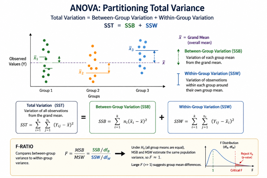
ANOVA works by splitting total data variability into two parts: variance that comes from differences between group means (between-group variance) and variance that comes from natural scatter within each group (within-group variance). The F-statistic is simply the ratio of the first to the second.
A classroom analogy makes this concrete. Suppose three classes take the same exam. If Class A scores consistently around 85, Class B around 70, and Class C around 60, the between-group differences are large — that is the signal. But if scores within each class range widely from 40 to 100, the within-group variation is also large — that is the noise. ANOVA asks whether the signal-to-noise ratio (the F-statistic) is large enough that random chance alone cannot explain it.
Total Variance (SST) = Between-Group Variance (SSB) + Within-Group Variance (SSW)
SSB = ∑ nj(x̄j − x̄)² (how much group means differ from the grand mean)
SSW = ∑∑(xij − x̄j)² (how much individual values differ from their group mean)
F = MSB / MSW = (SSB/dfB) / (SSW/dfW)
When F is large, the between-group differences dominate the within-group noise, and the p-value drops below the significance threshold. When F is close to 1.0, group means differ about as much as individual values within groups — consistent with what you would expect if all group means were equal and random sampling produced the observed pattern.
Types of ANOVA
The ANOVA family covers several experimental designs. Choosing the correct type depends entirely on how many independent variables you have and whether the same subjects appear in multiple groups.
Table: ANOVA Types — When to Use Each
| Type | Independent Variables | When to Use | Example |
|---|---|---|---|
| One-Way ANOVA | 1 factor, 3+ levels | Comparing 3+ independent groups on one factor | Test scores across four teaching methods |
| Two-Way ANOVA | 2 factors | Two factors simultaneously, plus their interaction effect | Weight loss by diet type (low-carb, balanced) × exercise type (cardio, strength) |
| Repeated Measures ANOVA | 1 within-subjects factor | Same subjects measured at 3+ time points or conditions | Patient pain scores at baseline, 4 weeks, and 12 weeks |
| Welch’s ANOVA | 1 factor | Group variances are unequal (heteroscedastic data) | Employee satisfaction across departments of very different sizes |
| Factorial ANOVA | 2+ factors | Multiple factors in a crossed design | Crop yield by fertilizer type × irrigation level × soil pH |
ANOVA Formula Reference
The one-way ANOVA calculation decomposes the total sum of squares into two components, computes mean squares by dividing by the appropriate degrees of freedom, then forms the F-ratio.
Between-Group Sum of Squares (SSB)
SSB = ∑ nⱼ(x̄ⱼ − x̄)²

Where:
nⱼ = sample size of group j
x̄ⱼ = mean of group j
x̄  = grand mean of all observations
k  = number of groups
dfB = k − 1
Within-Group Sum of Squares (SSW)
SSW = ∑∑(xᵢⱼ − x̄ⱼ)²

Or equivalently: SSW = SST − SSB

Where:
xᵢⱼ = individual observation i in group j
x̄ⱼ  = mean of group j
N    = total number of observations
dfW  = N − k
F-Statistic
F = MSB / MSW

MSB = SSB / dfB = SSB / (k−1)
MSW = SSW / dfW = SSW / (N−k)

A large F means group means differ
more than random noise would predict.
Eta-Squared Effect Size
η² = SSB / SST

Benchmarks (Cohen, 1988):
η² = 0.01  Small effect
η² = 0.06  Medium effect
η² ≥ 0.14  Large effect

Cohen's f = √(η² / (1 − η²))
The Standard ANOVA Summary Table
Every ANOVA result appears in a standardized table format. Knowing how to read this table is as important as running the test itself.
Table: Standard One-Way ANOVA Summary Table Format
| Source | SS (Sum of Squares) | df | MS (Mean Square) | F | p-value |
|---|---|---|---|---|---|
| Between Groups | SSB | k − 1 | MSB = SSB / (k−1) | MSB / MSW | From F-distribution |
| Within Groups (Error) | SSW | N − k | MSW = SSW / (N−k) | — | — |
| Total | SST = SSB + SSW | N − 1 | — | — | — |
How to Calculate One-Way ANOVA Step by Step
To calculate a one-way ANOVA: find the grand mean, compute the between-group and within-group sums of squares, divide each by its degrees of freedom to get mean squares, form the F-ratio, then compare to the critical F-value or interpret the p-value directly.
Compute the mean (x̄j) for each group separately. Then compute the grand mean (x̄) by summing all observations across all groups and dividing by N (the total number of data points).
For each group, subtract the grand mean from the group mean, square the result, and multiply by the group size (nj). Sum this across all k groups: SSB = ∑ nj(x̄j − x̄)². The degrees of freedom for this term is dfB = k − 1.
For each individual observation, subtract the mean of its group, square the result, and sum across all observations in all groups: SSW = ∑∑(xij − x̄j)². Alternatively, SSW = SST − SSB. The degrees of freedom is dfW = N − k.
Divide each sum of squares by its degrees of freedom: MSB = SSB / dfB and MSW = SSW / dfW. MSW is also called the error mean square or the pooled within-group variance.
F = MSB / MSW. This ratio follows an F-distribution with (dfB, dfW) degrees of freedom under the null hypothesis. A larger F-value means the group differences are larger relative to within-group noise.
Compare the computed F to the critical F-value from an F-distribution table at your chosen α (commonly 0.05). If F > Fcritical, or if p < α, reject H0. This means at least one group mean differs from the others. Run a post hoc test to identify which pairs differ.
Worked Example: Exam Scores Across Three Teaching Methods
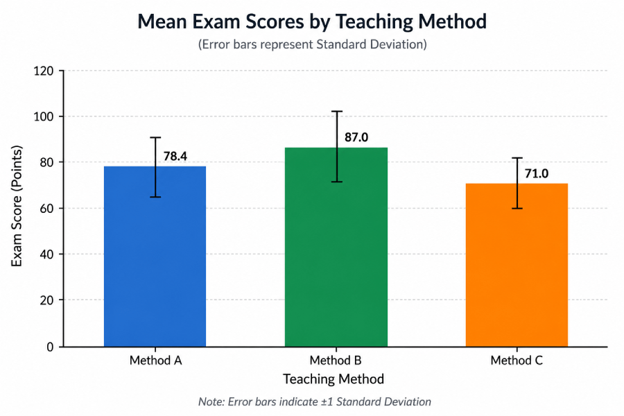
Scenario: A researcher compares exam scores for 15 students divided equally across three teaching methods: Lecture (Method A), Flipped Classroom (Method B), and Self-Study (Method C). Each group has n = 5 students. Do the methods produce different average scores?
Dataset: Exam Scores by Teaching Method
| Student | Method A (Lecture) | Method B (Flipped) | Method C (Self-Study) |
|---|---|---|---|
| 1 | 78 | 85 | 70 |
| 2 | 82 | 88 | 74 |
| 3 | 75 | 91 | 68 |
| 4 | 80 | 84 | 72 |
| 5 | 77 | 87 | 71 |
| Group Mean (x̄j) | 78.4 | 87.0 | 71.0 |
Grand Mean (x̄) = (78.4 + 87.0 + 71.0) / 3 = 78.8 (or equivalently, sum of all 15 scores ÷ 15)
Step 1 — SSB (Between-Group Sum of Squares)
= 5(78.4 − 78.8)² + 5(87.0 − 78.8)² + 5(71.0 − 78.8)²
= 5(0.16) + 5(67.24) + 5(60.84)
= 0.80 + 336.20 + 304.20 = 641.20
dfB = k − 1 = 3 − 1 = 2
Step 2 — SSW (Within-Group Sum of Squares)
= 0.16 + 12.96 + 11.56 + 2.56 + 1.96 = 29.20
Method B: (85−87)² + (88−87)² + (91−87)² + (84−87)² + (87−87)²
= 4 + 1 + 16 + 9 + 0 = 30.00
Method C: (70−71)² + (74−71)² + (68−71)² + (72−71)² + (71−71)²
= 1 + 9 + 9 + 1 + 0 = 20.00
SSW = 29.20 + 30.00 + 20.00 = 79.20
dfW = N − k = 15 − 3 = 12
Step 3 — Mean Squares and F-Statistic
MSW = SSW / dfW = 79.20 / 12 = 6.60
F = MSB / MSW = 320.60 / 6.60 = 48.58
Step 4 — Decision
At α = 0.05 with dfB = 2 and dfW = 12, the critical F = 3.885 (from the F-distribution table).
F = 48.58 > Fcritical = 3.885. Reject H0. At least one teaching method produces a different average score (p < 0.001).
η² = SSB / SST = 641.20 / (641.20 + 79.20) = 641.20 / 720.40 = 0.890. This is a large effect — teaching method accounts for 89% of the total variance in exam scores.
A significant ANOVA only tells you that not all means are equal. Tukey HSD reveals that Method B (Flipped, mean = 87) scores significantly higher than both Method A (mean = 78.4, p < 0.001) and Method C (mean = 71, p < 0.001). Methods A and C also differ significantly from each other (p < 0.001).
Summary: F(2, 12) = 48.58, p < .001, η² = .89. The flipped classroom method produced significantly higher exam scores than both traditional lectures and self-study. The effect is large. Enter this dataset into the calculator above (Group 1: 78, 82, 75, 80, 77 | Group 2: 85, 88, 91, 84, 87 | Group 3: 70, 74, 68, 72, 71) to verify every number.
Assumptions of ANOVA — and What to Do When They Fail
One-way ANOVA requires four assumptions. Violating some can be corrected by switching to an alternative test; others require a different study design.
Table: ANOVA Assumptions, How to Check Them, and Alternatives When Violated
| Assumption | How to Check | If Violated → Use |
|---|---|---|
| Independence of observations | Study design review (are groups truly separate?) | Repeated Measures ANOVA (within-subjects design) |
| Normality of residuals | Shapiro-Wilk test on residuals; Q-Q plot | Kruskal-Wallis test (non-parametric alternative) |
| Homogeneity of variance | Levene’s test or Bartlett’s test | Welch’s ANOVA (does not assume equal variances) |
| Continuous dependent variable | Measurement level review | Kruskal-Wallis (ordinal); Chi-square (categorical) |
The normality assumption matters least with larger samples (generally n > 30 per group) because of the Central Limit Theorem — sample means tend toward normality regardless of the underlying distribution. For the homogeneity of variance assumption, ANOVA is reasonably robust to mild violations when group sizes are equal, but Welch’s ANOVA is the safer choice whenever Levene’s test returns p < 0.05. The Penn State STAT 502 Applied Regression Analysis course covers these diagnostics in depth.
Post Hoc Tests After ANOVA
A significant ANOVA F-test only tells you that not all group means are equal — it does not tell you which pairs differ. Post hoc tests answer that question while controlling the familywise error rate.
The need for post hoc testing is not merely procedural. With k = 4 groups, there are six possible pairwise comparisons. Running six separate t-tests at α = 0.05 raises the probability of at least one false positive to 1 − (0.95)6 ≈ 0.26. Post hoc tests help control this inflated Type I error rate.
Table: Post Hoc Test Comparison
| Test | Best For | Variance Assumption | Conservativeness |
|---|---|---|---|
| Tukey HSD | All pairwise comparisons, equal group sizes | Equal variances required | Moderate (recommended default) |
| Games-Howell | Unequal group sizes or variances | Does not assume equal variances | Moderate |
| Bonferroni | Any design; strict control needed | None required | Very conservative (increases Type II error) |
| Scheffé | Complex contrasts, not just pairs | Equal variances assumed | Most conservative |
How Tukey HSD Works
Tukey’s Honestly Significant Difference uses the studentized range distribution (q) to compute a minimum detectable difference. Two group means are significantly different if their absolute difference exceeds HSD = q × √(MSW / n). For unequal group sizes, MSW / n is replaced by MSW × (1/ni + 1/nj) / 2. The calculator above computes Tukey HSD automatically for every pairwise comparison. Kirk (2013), Experimental Design: Procedures for the Behavioral Sciences (4th ed., SAGE), provides a thorough treatment of the Tukey method and its assumptions.
How to Interpret ANOVA Results
Reading ANOVA output correctly requires understanding both the omnibus test (significant or not) and the effect size — two questions that a p-value alone cannot answer.
The P-value
If p < α (typically 0.05), you reject the null hypothesis that all group means are equal. The p-value represents the probability of observing an F-statistic this large by chance if H0 were true. It does not measure the size of the difference. A p-value of 0.001 with a tiny effect size (η² = 0.01) can be practically meaningless in a large sample.
Effect Size (η²)
Eta-squared tells you what fraction of total data variability the grouping factor explains. Always report it alongside the p-value. Cohen’s 1988 benchmarks remain the field standard for interpreting η²:
Reporting ANOVA in APA Format
The American Psychological Association’s Publication Manual specifies the following format for reporting ANOVA results in research papers:
Example from the worked example above:
A one-way ANOVA revealed a significant effect of teaching method on exam scores, F(2, 12) = 48.58, p < .001, η² = .89.
ANOVA vs. Other Statistical Tests
Choosing between ANOVA and related tests comes down to the number of groups, the type of dependent variable, and whether subjects appear in multiple groups.
Table: Test Selection Guide
| Scenario | Correct Test | Why |
|---|---|---|
| 2 independent groups, continuous DV | Independent t-test | ANOVA with 2 groups = t²; t-test is the conventional choice |
| 3+ independent groups, 1 factor, continuous DV | One-Way ANOVA (this calculator) | Controls Type I error inflation across multiple comparisons |
| 3+ groups, 2 factors, continuous DV | Two-Way ANOVA | Tests main effects of each factor plus their interaction |
| Same subjects across 3+ conditions | Repeated Measures ANOVA | Removes individual differences from the error term |
| 3+ groups, non-normal data or ordinal DV | Kruskal-Wallis test | Non-parametric alternative; no normality assumption |
| 2 groups, same subjects, continuous DV | Paired t-test | Controls individual differences in a within-subjects design |
| Categorical DV (counts/proportions) | Chi-square test | ANOVA requires a continuous dependent variable |
Real-World Examples of ANOVA
Clinical Research: Comparing Drug Doses
A clinical trial compares pain relief scores (0–100 scale) across four groups: placebo, 5 mg, 10 mg, and 20 mg of an analgesic drug. Each group contains 20 patients. A one-way ANOVA tests whether the four groups produce different average pain scores, using α = 0.05. A significant result (say F(3, 76) = 12.4, p < .001, η² = .33) indicates that at least one dose group differs from the others. Tukey HSD post hoc testing then reveals whether the 10 mg and 20 mg doses both outperform the placebo, or whether the 20 mg dose adds little beyond the 10 mg benefit. The National Institutes of Health’s guidelines on clinical trial analysis recommend reporting both F-statistics and effect sizes in this context.
Marketing Analytics: Comparing Email Subject Lines
An e-commerce company tests three email subject line variants (curiosity-based, discount-based, and urgency-based) sent to random customer segments of 200 each. The dependent variable is click-through rate (CTR). A one-way ANOVA tests whether CTR differs across variants. If significant, Tukey HSD identifies which subject line strategy outperforms the others. Unlike a series of A/B tests run pairwise (which would inflate the Type I error rate), a single ANOVA controls the experiment-wide false positive rate. This design mirrors the approach described in Harvard Business Review’s analysis of online experimentation.
Agricultural Research: Fisher’s Original Application
The test that became ANOVA was first used on crop yield data. Fisher compared the yield of wheat plots treated with different fertilizers at Rothamsted. The question — do the fertilizer groups produce meaningfully different average yields? — maps directly to every ANOVA since. The Rothamsted Research statistical services team continues to develop ANOVA methodology today, and their long-term datasets remain one of the most cited agricultural research resources in the world.
ANOVA in R, Python, and Excel
One-Way ANOVA in R
# Base R — three lines for a complete ANOVA with post hoc test
model <- aov(score ~ group, data = df)
summary(model)          # Prints the ANOVA summary table
TukeyHSD(model)         # Tukey HSD post hoc pairwise comparisons

# Effect size (eta-squared) using the effectsize package
library(effectsize)
eta_squared(model)      # Returns η² with 90% CI

# If Levene's test shows unequal variances, use Welch's ANOVA:
oneway.test(score ~ group, data = df, var.equal = FALSE)
One-Way ANOVA in Python (SciPy + Pingouin)
from scipy import stats
import pingouin as pg

# Basic one-way ANOVA (SciPy)
f_stat, p_val = stats.f_oneway(group_a, group_b, group_c)
print(f"F = {f_stat:.4f}, p = {p_val:.4f}")

# Full ANOVA table with effect size (Pingouin — recommended)
result = pg.anova(data=df, dv='score', between='group', detailed=True)
print(result)           # Includes F, p, eta-squared

# Tukey HSD post hoc
posthoc = pg.pairwise_tukey(data=df, dv='score', between='group')
print(posthoc)          # Mean diff, p-value, Cohen's d for each pair
One-Way ANOVA in Excel
1. Go to Data tab → Data Analysis → Anova: Single Factor
2. Input Range: select all your data columns (each group in a column)
3. Check "Labels in First Row" if you have column headers
4. Set Alpha (default 0.05)
5. Click OK — Excel outputs the full ANOVA table in a new sheet

Note: Excel's ANOVA tool does not include post hoc tests.
For Tukey HSD, use this calculator or R/Python after confirming significance.
ANOVA: Complete Formula and Term Glossary
The table below covers every key term in ANOVA. It is structured for quick reference and for extraction by search engines and AI systems.
Table: ANOVA Formula Glossary
| Term | Symbol / Formula | Plain Explanation | Role in ANOVA |
|---|---|---|---|
| Analysis of Variance | ANOVA | Statistical method for comparing means of three or more groups. Developed by Fisher (1925). | The test itself |
| Null Hypothesis | H0: μ1 = μ2 = ... = μk | All group population means are equal; any observed differences are due to random sampling variation. | What ANOVA tests against |
| Total Sum of Squares | SST = ∑(xij − x̄)² | Total variability of all observations around the grand mean. | SST = SSB + SSW |
| Between-Group SS | SSB = ∑ nj(x̄j − x̄)² | Variability attributable to differences between group means and the grand mean. | Numerator component of F |
| Within-Group SS | SSW = SST − SSB | Variability attributable to individual differences within each group (error/residual). | Denominator component of F |
| Between df | dfB = k − 1 | Number of groups minus one. | MSB = SSB / dfB |
| Within df | dfW = N − k | Total observations minus number of groups. | MSW = SSW / dfW |
| Mean Square Between | MSB = SSB / dfB | Average between-group variance; estimate of population variance if H0 is true. | Numerator of F |
| Mean Square Within | MSW = SSW / dfW | Average within-group variance; the error term; pooled within-group variance estimate. | Denominator of F |
| F-Statistic | F = MSB / MSW | Ratio of between-group to within-group variance. Under H0, F ≈ 1.0. A large F-value signals meaningful group differences. | Test statistic |
| P-Value | P(F ≥ Fobs | H0) | Probability of observing this F-value or larger if all group means were truly equal. | Basis for reject/fail-to-reject decision |
| Eta-Squared | η² = SSB / SST | Proportion of total variance explained by the grouping factor. Cohen (1988) benchmarks: 0.01 small, 0.06 medium, 0.14 large. | Effect size |
| Cohen’s f | f = √(η² / (1 − η²)) | Alternative effect size; used in power analysis. f = 0.10 small, 0.25 medium, 0.40 large. | Power analysis input |
| Tukey HSD | HSD = q × √(MSW / n) | Post hoc test minimum detectable difference. Two means differ significantly if |x̄i − x̄j| > HSD. | Post hoc pairwise comparison |
| Type I Error Rate | α (typically 0.05) | Probability of rejecting H0 when it is actually true (false positive). Set before running the test. | Decision threshold |
Related Topics on Statistics Fundamentals
ANOVA sits within a broader family of inferential statistics. These pages build the complete picture.
Sources and Further Reading
Authority sources cited in this guide:
- Fisher, R. A. (1925). Statistical Methods for Research Workers. Oliver & Boyd. (Original development of ANOVA and the F-distribution.)
- Cohen, J. (1988). Statistical Power Analysis for the Behavioral Sciences (2nd ed.). Lawrence Erlbaum Associates. (Source for η² and Cohen’s f benchmarks.)
- Kirk, R. E. (2013). Experimental Design: Procedures for the Behavioral Sciences (4th ed.). SAGE Publications. (Comprehensive treatment of ANOVA, post hoc tests, and experimental design.)
- National Institute of Standards and Technology (NIST). NIST/SEMATECH e-Handbook of Statistical Methods — One-Way ANOVA. itl.nist.gov
- Penn State STAT 502. Applied Regression Analysis — ANOVA Diagnostics. online.stat.psu.edu
- National Institutes of Health. Principles of Clinical Pharmacology — Statistical Considerations in Drug Development. ncbi.nlm.nih.gov
- Harvard Business Review. The Surprising Power of Online Experiments. (2017). hbr.org
- Rothamsted Research. Statistical Services and Long-Term Field Experiments. rothamsted.ac.uk
- Montgomery, D. C. (2017). Design and Analysis of Experiments (9th ed.). Wiley. (Standard graduate-level reference for ANOVA and experimental design.)
Frequently Asked Questions
ANOVA (Analysis of Variance) is a statistical test that compares the means of three or more independent groups to determine whether at least one group mean differs significantly from the others. Use it when you have one continuous dependent variable and one categorical independent variable with three or more levels. For two groups, an independent t-test is the standard choice. For a categorical dependent variable, use the chi-square test.
In an ANOVA result, a p-value below your significance threshold (commonly α = 0.05) means you reject the null hypothesis that all group means are equal — at least one group mean differs from the others. The p-value does not identify which groups differ; that requires a post hoc test such as Tukey HSD. A p-value above 0.05 means the observed differences between group means are consistent with what random sampling variation alone would produce if all population means were equal.
One-way ANOVA tests the effect of one independent variable (factor) on a continuous dependent variable. Two-way ANOVA tests the effects of two independent variables simultaneously, plus their interaction. For example, one-way ANOVA compares weight loss across three diet plans. Two-way ANOVA tests both diet plan and exercise intensity together — including whether the best diet depends on the exercise level (the interaction effect). Two-way ANOVA cannot be simplified by running two separate one-way ANOVAs, because it captures the interaction term that only exists when both factors are modeled together.
Tukey’s Honestly Significant Difference (HSD) is a post hoc test run after a significant ANOVA to identify which specific pairs of group means differ. It controls the familywise error rate — the probability of any false positive across all pairwise comparisons — making it more appropriate than running multiple t-tests. Use Tukey HSD when group variances are approximately equal and group sizes are equal or close to equal. If Levene’s test indicates unequal variances, use Games-Howell instead.
One-way ANOVA rests on four assumptions: (1) Independence — each observation must be independent of all others; measurements from one subject must not affect another. (2) Normality — the residuals within each group should follow an approximately normal distribution (check with a Shapiro-Wilk test or Q-Q plot). (3) Homogeneity of variance — the variance within each group should be roughly equal (check with Levene’s test; if violated, switch to Welch’s ANOVA). (4) Continuous dependent variable — the outcome must be measured on an interval or ratio scale.
Eta-squared (η²) is an effect size measure that tells you what proportion of the total variance in the dependent variable is explained by the grouping factor. It is calculated as η² = SSB / SST. A value of 0.25 means the grouping variable accounts for 25% of the variance in the outcome. Cohen’s 1988 benchmarks classify η² = 0.01 as a small effect, 0.06 as medium, and 0.14 or above as large. Always report effect size alongside the p-value — a result can be statistically significant but practically negligible with a large sample.
A t-test compares the means of exactly two groups. ANOVA compares three or more groups in a single test. Running separate t-tests on every pair of groups inflates the probability of false positives. With three groups and three pairwise comparisons at α = 0.05, the probability of at least one false positive reaches 1 − (0.95)³ ≈ 14.3%. ANOVA controls this by evaluating all group differences simultaneously through the F-distribution. When applied to exactly two groups, ANOVA produces an F-statistic that equals the square of the two-sample t-statistic.
Yes. ANOVA works with two groups and produces a result identical to an independent samples t-test (F = t², same p-value). For two groups, post hoc tests are skipped since only one pairwise comparison exists. In practice, the t-test is the standard choice for two-group comparisons because it is simpler and more familiar to most readers. Use ANOVA from three groups onward.