What Is Standard Deviation? (Simple Definition)
Think of standard deviation as the "average distance" each data point travels from the center. If you recorded the daily commute times of 20 people who all live in the same neighborhood, and every single one takes exactly 25 minutes, the standard deviation is zero — nobody deviates from the average at all. But if commutes range from 10 minutes to 65 minutes, the SD would be large, telling you the data is highly variable.
Standard deviation is arguably the most important single-number summary of variability in statistics. According to the NIST/SEMATECH e-Handbook of Statistical Methods, the standard deviation is the primary measure of spread used in descriptive statistics, quality engineering, and hypothesis testing. Every branch of descriptive statistics relies on it as a foundation. The team at Statistics Fundamentals has built this guide to make that foundation solid.
- Symbol: σ (sigma) for population; s for sample
- Population formula: σ = √[Σ(xᵢ − μ)² / N]
- Sample formula: s = √[Σ(xᵢ − x̄)² / (n − 1)]
- Can it be negative? Never — SD is always ≥ 0; it equals 0 only when all values are identical
- Units: Same as the original data (e.g., kilograms, dollars, seconds)
- 68-95-99.7 rule: In a normal distribution, ~68% of data falls within ±1 SD; ~95% within ±2 SD; ~99.7% within ±3 SD
The Standard Deviation Formula (Population vs. Sample)
There are two versions of the standard deviation formula, and choosing the wrong one introduces systematic error. The distinction depends on whether your data represents an entire group or just a subset of a larger group.
Population Standard Deviation: σ = √[Σ(xᵢ − μ)² / N]
σ = population standard deviation (sigma)
xᵢ = each individual data point
μ = population mean (mu)
N = total number of values in the population
Σ = sum of all values
Apply the population formula when you have every single data point for the group you are measuring. For example: the exam scores of all 30 students in a specific class, the daily revenue of a single restaurant across an entire year, or the heights of every player on one basketball team. When you have the complete picture, divide by N.
Sample Standard Deviation: s = √[Σ(xᵢ − x̄)² / (n − 1)]
s = sample standard deviation
xᵢ = each individual data point
x̄ = sample mean (x-bar)
n = number of values in the sample
n − 1 = Bessel's correction for bias
The n − 1 denominator is called Bessel's correction. When you use a sample mean (x̄) instead of the true population mean (μ), the deviations tend to be slightly smaller than the real deviations from μ — this underestimates the true spread. Dividing by n − 1 instead of n inflates the result just enough to correct that bias. Penn State's STAT 500 course notes confirm this: dividing by n produces a biased estimator of σ, while dividing by n − 1 produces an unbiased estimator (Penn State STAT 500).
Ask yourself: "Do I have every single value in the group?" If yes → use σ (divide by N). If you collected data from a subset and want to draw conclusions about a larger group → use s (divide by n − 1). In most real-world research, surveys, and data science work, you are almost always working with a sample.
How to Calculate Standard Deviation: Step by Step
Step 1: Find the mean. Step 2: Subtract the mean from each value (find each deviation). Step 3: Square each deviation. Step 4: Sum the squared deviations. Step 5: Divide by N (population) or n − 1 (sample) to get the variance. Step 6: Take the square root — that is your standard deviation.
Worked Example 1 — Small Dataset (5 Test Scores)
Five students take a quiz and score: 72, 85, 90, 68, 95. Calculate the sample standard deviation.
Find the mean (x̄): (72 + 85 + 90 + 68 + 95) / 5 = 410 / 5 = 82
Find each deviation (xᵢ − x̄): 72−82 = −10 | 85−82 = 3 | 90−82 = 8 | 68−82 = −14 | 95−82 = 13
Square each deviation: (−10)² = 100 | 3² = 9 | 8² = 64 | (−14)² = 196 | 13² = 169
Sum the squared deviations: 100 + 9 + 64 + 196 + 169 = 538
Divide by n − 1 (sample variance): 538 / (5 − 1) = 538 / 4 = 134.5
Take the square root: s = √134.5 ≈ 11.60
✓ The sample standard deviation is approximately 11.60 points. This means the typical quiz score deviates from the class average of 82 by about 11.6 points in either direction.
The table below shows every calculation column by column — the format you will use in exams and statistics software output:
| Student | Score (xᵢ) | Deviation (xᵢ − 82) | Squared Dev. (xᵢ − 82)² |
|---|---|---|---|
| A | 72 | −10 | 100 |
| B | 85 | 3 | 9 |
| C | 90 | 8 | 64 |
| D | 68 | −14 | 196 |
| E | 95 | 13 | 169 |
| Sum of Squared Deviations | 538 | ||
| Sample Variance (÷ n−1 = 4) | 134.5 | ||
| Sample SD (√134.5) | ≈ 11.60 | ||
Worked Example 2 — Population Standard Deviation (Manufacturing)
A machine produces exactly 6 bolts per run. Their diameters in mm are: 10.1, 9.9, 10.3, 10.0, 9.8, 10.2. These are all bolts produced — compute the population SD.
Mean (μ): (10.1 + 9.9 + 10.3 + 10.0 + 9.8 + 10.2) / 6 = 60.3 / 6 = 10.05 mm
Squared deviations: (0.05)² + (−0.15)² + (0.25)² + (−0.05)² + (−0.25)² + (0.15)² = 0.0025 + 0.0225 + 0.0625 + 0.0025 + 0.0625 + 0.0225 = 0.175
Population variance (÷ N = 6): 0.175 / 6 ≈ 0.02917
Population SD (√0.02917): σ ≈ 0.171 mm
✓ σ ≈ 0.171 mm. The bolt diameters deviate from target by an average of 0.171mm. In a Six Sigma quality process, this would be compared against engineering tolerance limits — if the tolerance is ±0.5mm, this machine operates well within spec (tolerance / σ ≈ 2.9σ).
If you sum the raw deviations (without squaring), you always get zero — positive and negative deviations cancel out perfectly. This is why squaring is not optional. The squaring step is what makes standard deviation mathematically meaningful.
🧮 Standard Deviation Calculator
Enter your numbers separated by commas. The calculator shows population SD, sample SD, mean, and variance — with a step-by-step breakdown.
For more advanced statistics, see the dedicated standard deviation calculator and the full descriptive statistics calculator on Statistics Fundamentals.
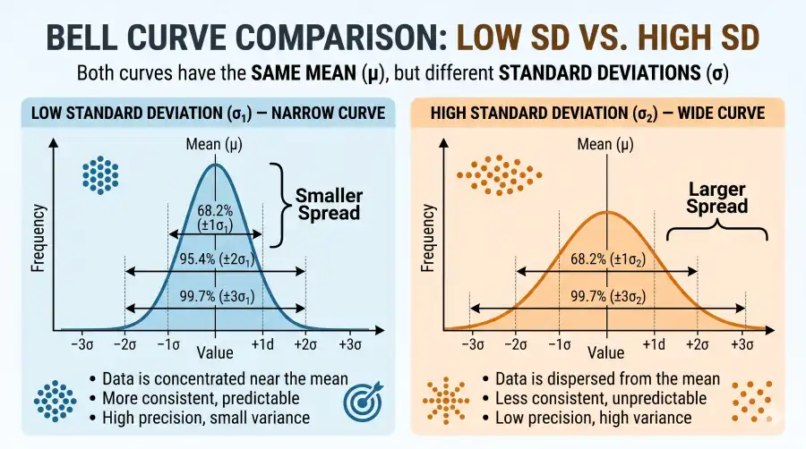
Standard Deviation and the Bell Curve: The 68-95-99.7 Rule
When data follows a normal distribution, standard deviation takes on a precise, predictable role. The empirical rule — also called the 68-95-99.7 rule — tells you exactly what percentage of data falls within 1, 2, and 3 standard deviations of the mean.
Standard Deviation Zones on the Normal Distribution (Bell Curve)
The central shaded band covers ±1σ (68.27% of normally distributed data). Each wider band adds roughly 13.5% on each side.
| SD Range | % of Data | IQ Example (μ=100, σ=15) | What It Means |
|---|---|---|---|
| μ ± 1σ | 68.27% | 85 to 115 | Most people — the "typical" range |
| μ ± 2σ | 95.45% | 70 to 130 | Covers nearly everyone; used for 95% confidence intervals |
| μ ± 3σ | 99.73% | 55 to 145 | Extreme outliers — only 0.27% of data falls outside this |
The empirical rule only applies to normally distributed data. For datasets with unknown or non-normal distributions, Chebyshev's inequality provides a weaker but universal guarantee: at least 75% of values always fall within ±2 SD, and at least 89% within ±3 SD, regardless of distribution shape. This is described in detail by Penn State's statistics curriculum.
Population vs. Sample Standard Deviation: Which Formula Do You Use?
This is the single most common source of confusion in introductory statistics courses. The short answer: when in doubt, use the sample formula. Here is exactly when to use each one.
| Criterion | Population SD (σ) | Sample SD (s) |
|---|---|---|
| Data represents | Every member of the entire group | A subset drawn from a larger group |
| Formula denominator | N (total count) | n − 1 (Bessel's correction) |
| Symbol | σ (sigma) | s |
| Excel function | =STDEV.P() | =STDEV.S() |
| Python (NumPy) | np.std(x, ddof=0) | np.std(x, ddof=1) |
| Common use cases | All students in one class; all products in one production run | Survey respondents; medical trial participants; polling data |
| Bias | Exact (no estimation needed) | Unbiased estimator of population σ |
If your data describes a complete group with no intention to generalize → σ (population). If your data was collected to make inferences about a larger group → s (sample). Research, polling, and most data science work almost always requires s.
Standard Deviation vs. Variance: Key Differences
Variance and standard deviation measure the same thing — spread — but differ in how they express it. Variance (σ²) is the average of squared deviations. Standard deviation (σ) is simply the square root of variance. The relationship is: σ² → take square root → σ.
| Property | Variance (σ²) | Standard Deviation (σ) |
|---|---|---|
| Formula | σ² = Σ(xᵢ − μ)² / N | σ = √[Σ(xᵢ − μ)² / N] |
| Units | Squared (e.g., dollars², kg²) | Same as data (e.g., dollars, kg) |
| Interpretability | Hard to interpret directly | Directly interpretable |
| Relationship | Variance = SD² | SD = √Variance |
| Used in | ANOVA, regression, theoretical proofs | Descriptive statistics, confidence intervals |
If a dataset of house prices has a standard deviation of $45,000, you can immediately say "prices typically deviate from average by about $45,000." If you use variance, you get $2,025,000,000 — mathematically correct but impossible to communicate intuitively. This is precisely why SD, not variance, is the preferred summary statistic in most reports and publications. For a deeper treatment of variance, see the statistics and probability section.
Standard Deviation vs. Standard Error: A Critical Distinction
This is one of the most frequently misunderstood distinctions in statistics — including in published scientific papers. Confusing SD and SE leads to systematically wrong confidence intervals and misleading results.
Standard deviation describes how much individual values vary within your dataset. Standard error describes how much sample means vary if you repeated your study many times.
SE = standard error of the mean
s = sample standard deviation
n = sample size
| Property | Standard Deviation (SD) | Standard Error (SE) |
|---|---|---|
| What it measures | Spread of individual data points | Precision of the sample mean |
| Formula | σ = √[Σ(xᵢ − μ)² / N] | SE = s / √n |
| Effect of larger n | Does not systematically decrease | Decreases — larger samples → more precise estimates |
| Used for | Describing data variability | Confidence intervals, hypothesis tests |
| Related to | Individual observations | Sampling distributions |
Multiple meta-analyses have found that approximately 25–30% of published biomedical papers confuse SD and SE in their reported summary statistics. Always check which one a paper is using before interpreting confidence intervals or effect sizes. The Altman and Bland (2005) British Medical Journal analysis documented this pattern extensively.
Z-Scores: Using Standard Deviation to Standardize Data
A z-score converts a raw data point into a unit that tells you how many standard deviations it sits from the mean. This allows comparison across completely different datasets and scales.
x = individual raw score
μ = mean of the distribution
σ = standard deviation
z = number of SDs from the mean
A student scores 91 on a history exam (μ = 78, σ = 9) and 74 on a math exam (μ = 65, σ = 6). Which performance was stronger relative to classmates?
History z-score: z = (91 − 78) / 9 = 13 / 9 ≈ 1.44
Math z-score: z = (74 − 65) / 6 = 9 / 6 = 1.50
✓ The math exam (z = 1.50) was the stronger relative performance — the student sat 1.5 SDs above the math mean vs. only 1.44 SDs above the history mean. Without standardizing using σ, comparing the raw scores of 91 and 74 is meaningless. Use the Z-score calculator to find percentile rankings instantly.
Real-World Standard Deviation Examples
Standard deviation is not a classroom-only concept. It is the backbone of financial risk models, quality engineering, clinical research, and sports analytics. Here are five concrete domain applications with realistic data.
Annual Return Volatility: S&P 500
The S&P 500 has produced an average annual return of roughly 10% over the past several decades, but with a standard deviation of approximately 15–18% per year. In practical terms, in about 68% of years, returns fall between roughly −8% and +28%. In the remaining 32% of years, returns fall outside that range — including crashes like 2008 (−37%) and explosive years like 2019 (+29%). Portfolio managers use SD as the primary metric for risk — higher SD means higher uncertainty, regardless of average return. This is the basis of Modern Portfolio Theory, developed by Harry Markowitz and described in full at Nobel Prize.org.
NBA Scoring: Consistency vs. Streakiness
Two NBA players both average 22 points per game. Player A has a game-by-game scoring SD of 4.2 points — they almost always score between 18 and 26 points. Player B has an SD of 11.8 points — they might score 8 points one night and 38 the next. Coaches value low-SD scorers for playoff reliability; fantasy sports analysts track high-SD players as "boom or bust" picks. Standard deviation is the statistic that separates these two identical averages into completely different player profiles.
SAT Score Spread and College Admissions
According to the College Board, the SAT has a total score mean of approximately 1060 and a standard deviation near 210. This means about 68% of test-takers score between 850 and 1270. A student scoring 1480 sits roughly two standard deviations above the mean — in approximately the 98th percentile. College admissions officers implicitly use this distribution when reading score ranges: a "mid-50% range" of 1300–1480 at a selective university represents roughly the 26th to 74th percentile within that school's applicant pool.
Why Six Sigma Is Called Six Sigma
Six Sigma is a quality control methodology where processes are designed so that specification limits sit six standard deviations from the process mean. At ±6σ, only 3.4 defects per million opportunities occur — a 99.99966% yield rate. Companies like Motorola and General Electric standardized this approach in the 1980s and 1990s. The NIST engineering statistics handbook covers the statistical basis of process capability at NIST PMC Section 1.6.
Temperature Consistency: San Francisco vs. Chicago
San Francisco has an average annual daily temperature around 57°F with a standard deviation near 5°F — temperatures are predictably mild year-round. Chicago has a similar annual average (~53°F) but a standard deviation exceeding 22°F, reflecting extreme variation between −10°F winter days and 95°F summer days. Same approximate mean; completely different lived experience. Standard deviation is what climate scientists use when comparing cities' temperature stability for agriculture, energy planning, and public health modeling.

How to Interpret Standard Deviation in Your Data
The number that comes out of the SD formula only becomes meaningful when you put it in context. Here are the three questions to ask every time you compute a standard deviation.
Question 1: What Are the Units?
SD is expressed in the same units as the original data. If you computed the SD of exam scores, the answer is in "points." If you computed the SD of household incomes, it is in dollars. A SD of 12 points is meaningless until you know the mean — if the mean is 15 points, a SD of 12 is enormous relative spread; if the mean is 500 points, it is negligible.
Question 2: What Is the Coefficient of Variation (CV)?
The coefficient of variation (CV = SD / mean × 100%) is a scale-free measure of relative variability. It lets you compare SD across datasets with different units or very different means:
- Dataset A: Mean = 100, SD = 15 → CV = 15%
- Dataset B: Mean = 1,000, SD = 80 → CV = 8%
- Despite Dataset B having a larger absolute SD, Dataset A is relatively more variable.
Question 3: Is the Data Normally Distributed?
If yes, use the empirical rule to interpret what the SD means in terms of probability. If the data is skewed or has heavy tails, the SD is still valid but the 68-95-99.7 percentages will not apply. For skewed data, consider pairing SD with a median and interquartile range when reporting descriptive statistics. See the mean and median guides on Statistics Fundamentals for choosing the right central tendency measure.
Standard Deviation in Excel, Python, and R
Every major statistics tool has a built-in SD function. The key is knowing which variant (population vs. sample) the default computes — they differ across software.
Excel: STDEV.S and STDEV.P
// Sample SD (divide by n−1) — USE THIS in most cases
=STDEV.S(A1:A20)
// Population SD (divide by N) — use when you have ALL data
=STDEV.P(A1:A20)
// Legacy functions (avoid — STDEV = STDEV.S, STDEVP = STDEV.P)
=STDEV(A1:A20) // same as STDEV.S
=STDEVP(A1:A20) // same as STDEV.P
Python: NumPy and Statistics Module
import statistics
data = [72, 85, 90, 68, 95]
# Sample SD (ddof=1 applies Bessel's correction) — most common
sample_sd = np.std(data, ddof=1)
print(f"Sample SD: {sample_sd:.4f}") # → 11.5975
# Population SD (ddof=0, the NumPy default)
pop_sd = np.std(data, ddof=0)
print(f"Population SD: {pop_sd:.4f}") # → 10.3682
# Using the statistics module (sample SD only)
print(statistics.stdev(data)) # → 11.5975 (sample)
print(statistics.pstdev(data)) # → 10.3682 (population)
np.std() defaults to ddof=0 (population SD). Most research and data science work requires the sample SD. Always specify ddof=1 in NumPy unless you explicitly have all population data. This catches many silent errors in data science code.
R: sd() Function
data <- c(72, 85, 90, 68, 95)
sd(data) # → 11.5975 (sample SD, n−1)
var(data) # → 134.5 (sample variance)
# For population SD in R:
sqrt(mean((data - mean(data))^2)) # → 10.3682 (population SD)
# Full descriptive statistics summary:
summary(data) # Min, Q1, Median, Mean, Q3, Max
sd(data) # Standard deviation
| Software | Sample SD (n−1) | Population SD (N) | Note |
|---|---|---|---|
| Excel | =STDEV.S(range) | =STDEV.P(range) | STDEV.S is the recommended modern function |
| Python (NumPy) | np.std(x, ddof=1) | np.std(x, ddof=0) | Default is ddof=0 (population) — specify ddof=1 for sample |
| Python (stats) | statistics.stdev(x) | statistics.pstdev(x) | statistics.stdev() always uses n−1 |
| R | sd(x) | Custom formula needed | R's sd() always uses n−1; no built-in psd() |
| Pandas (Python) | df['col'].std() | df['col'].std(ddof=0) | Pandas default is ddof=1 (sample) |
Formula & Concept Glossary
Every concept in this guide is connected. The glossary below defines each term precisely and shows how it relates to standard deviation — optimized for quick reference and study.
| Term | Formula | Plain-English Definition | Why It Matters |
|---|---|---|---|
| Standard Deviation | σ = √[Σ(xᵢ−μ)²/N] | Average distance each data point sits from the mean | Primary measure of variability in any dataset |
| Variance | σ² = Σ(xᵢ−μ)²/N | Average of squared deviations from the mean | Mathematical foundation of SD; used in ANOVA and regression |
| Mean | μ = Σxᵢ/N | Sum of all values divided by count — the arithmetic average | The reference point from which all deviations are measured |
| Median | Middle value (ordered) | The value that splits sorted data exactly in half | Better than mean for skewed data; not affected by outliers |
| Z-Score | z = (x−μ)/σ | How many standard deviations a value sits from the mean | Standardizes data for comparison across different scales |
| Standard Error | SE = s/√n | SD of the sampling distribution of means | Quantifies precision of a sample mean estimate |
| Normal Distribution | f(x) = (1/σ√2π)e^[−(x−μ)²/2σ²] | Symmetric bell-shaped distribution defined entirely by μ and σ | Enables the 68-95-99.7 rule; foundation of inferential statistics |
| Central Limit Theorem | (theorem — no single formula) | As sample size grows, sample means approach a normal distribution | Justifies using normal-based methods on non-normal populations |
| Confidence Interval | CI = x̄ ± z*(s/√n) | A range of values likely to contain the true population parameter | Translates statistical uncertainty into practical decision bounds |
| Coeff. of Variation | CV = (σ/μ) × 100% | SD expressed as a percentage of the mean | Allows SD comparisons across datasets with different units or scales |
Common Standard Deviation Mistakes (and How to Avoid Them)
| Mistake | What People Do | What's Correct |
|---|---|---|
| Wrong formula for context | Using σ (÷N) for a sample drawn from a population | Use s (÷n−1) for any sample that estimates a population parameter |
| Skipping the square step | Summing raw deviations (always gives zero) | Square each deviation before summing to eliminate cancellation |
| Confusing SD with SE | Using SD in a confidence interval formula instead of SE | CI uses SE = s/√n, not the raw SD of individual values |
| Interpreting SD without mean | "The SD is 15 — that's high" | SD of 15 with mean=20 is very high; with mean=1000 it's tiny. Always state both. |
| NumPy default assumption | Using np.std(x) and assuming it gives sample SD | np.std(x) gives population SD by default; add ddof=1 for sample SD |
| Applying the 68-95-99.7 rule to non-normal data | Assuming 68% of all datasets fall within ±1 SD | The empirical rule only applies to normally distributed data; use Chebyshev's inequality for all other distributions |
Standard Deviation in Hypothesis Testing and Confidence Intervals
Standard deviation connects directly to inferential statistics. The two most practical connections are confidence intervals and hypothesis testing.
Confidence Intervals
A 95% confidence interval for a population mean is computed as: CI = x̄ ± 1.96 × (s / √n). The standard deviation appears here in the standard error term (s / √n), which determines how wide the interval is. Smaller SD or larger sample size → narrower interval → more precise estimate of the true mean.
Z-Tests and T-Tests
In a one-sample t-test, the test statistic is t = (x̄ − μ₀) / (s / √n). The sample SD appears in the denominator. A larger SD inflates the denominator, reduces the test statistic, and makes it harder to detect a real effect — this is why underpowered studies with high variability often fail to reach statistical significance even when a true effect exists. The MIT OpenCourseWare statistics curriculum covers this trade-off in detail at MIT OCW 18.650.
Frequently Asked Questions About Standard Deviation
NIST/SEMATECH. (2012). e-Handbook of Statistical Methods — Measures of Scale. itl.nist.gov | Penn State STAT 500. Applied Statistics: Estimation. online.stat.psu.edu | Altman, D.G. & Bland, J.M. (2005). Standard deviations and standard errors. British Medical Journal. PMC1255808 | MIT OpenCourseWare. (2016). 18.650 Statistics for Applications. ocw.mit.edu | Moore, D.S., McCabe, G.P., & Craig, B.A. (2017). Introduction to the Practice of Statistics (9th ed.). W.H. Freeman.