The Shape Language of Data
The mean tells you where the center of your data sits. The standard deviation tells you how spread out the values are. These two numbers summarize most distributions well enough for everyday use — but they say nothing about shape.
Shape matters. A distribution can be symmetric or lopsided, can have thin tails or thick ones, can have most of its weight near the center or concentrated in the extremes. Two datasets with identical means and standard deviations can behave completely differently in practice. According to the NIST/SEMATECH Engineering Statistics Handbook, the third and fourth standardized moments — skewness and kurtosis — are the primary tools for detecting departures from normality and for understanding the shape of a distribution beyond its center and spread.
This is the full guide to both measures from Statistics Fundamentals. Each concept is covered in its own section, with formulas, examples, and the key differences between them. A glossary and FAQ follow the main content.
What is Skewness? (Direction of Data)
The formula above expresses skewness as the third standardized moment. In words: take every value's deviation from the mean, cube it (which preserves the sign, unlike squaring), average those cubed deviations, and divide by the cubed standard deviation to make the result unitless. The cube operation is what gives skewness its directional sensitivity — positive cubed deviations and negative cubed deviations do not cancel the way squared ones do.
g₁ = sample skewness
n = sample size
xᵢ = each data point
x̄ = sample mean
s = sample standard deviation
Most statistical software — including SPSS and Excel's SKEW() function — uses this Fisher–Pearson formulation. The correction factor n / ((n−1)(n−2)) matters most for small datasets. For large samples it approaches 1 and the simpler population formula gives essentially the same result.
A skewness value between −0.5 and +0.5 is generally considered approximately symmetric. Values between ±0.5 and ±1.0 indicate moderate skewness. Values beyond ±1.0 indicate substantial skewness that materially affects how you should interpret the mean. These thresholds are conventions, not laws — always look at a histogram alongside the number.
Positive Skew (Right-Skewed Data)
Long tail extends right
Most data clusters on the left; a smaller number of very high values stretches the distribution rightward. The mean is pulled above the median.
Mean > Median > Mode
The extreme values in the right tail inflate the mean. The median is a more reliable summary of a typical value in this case.
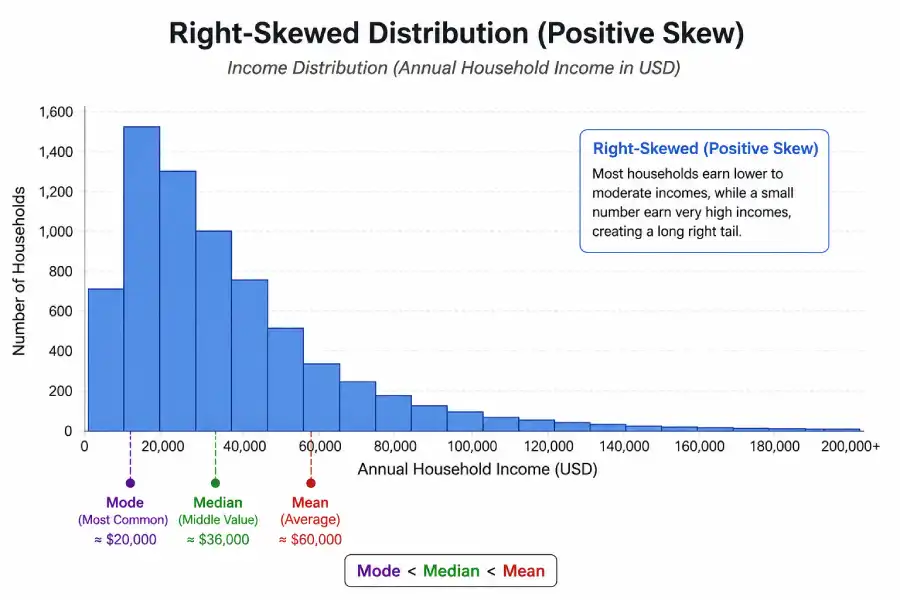
Income distribution in most countries shows clear positive skewness. The majority of households earn near the median — for the United States, the Census Bureau reports a consistent 20–25% gap between mean and median household income because a smaller number of very high earners pulls the mean upward. Using the mean to describe "typical" income in this context produces a misleading picture. Other common examples include housing prices, wealth distribution, and waiting times for rare events.
U.S. Household Income (Positive Skew)
According to the U.S. Census Bureau's Current Population Survey, the 2023 mean household income was approximately $105,000 while the median was around $77,000 — a gap of nearly $28,000. This difference is a direct consequence of the right-skewed income distribution. The mean is being pulled upward by households earning several hundred thousand dollars or more per year. The median better represents what a randomly selected household actually earns.
Negative Skew (Left-Skewed Data)
Long tail extends left
Most data clusters on the right; a smaller number of very low values pulls the distribution leftward. The mean falls below the median.
Mean < Median < Mode
The extreme low values in the left tail drag the mean downward. The median resists this distortion.
Negatively skewed distributions appear wherever there is a natural ceiling. Human lifespan in high-income countries is left-skewed: most people survive into their 70s or 80s, while a smaller number die young and pull the mean below the most common life expectancy. Easy exam scores — where most students score in the 80s and 90s — produce the same shape. Retirement age data and the time taken to complete a well-understood task both tend to be left-skewed for similar reasons.
Zero Skew (Symmetry)
A skewness of zero describes a distribution that is perfectly symmetric around its mean. The normal distribution is the most familiar example: its bell curve is a mirror image on either side of the mean, and mean = median = mode all sit at the same point. Many biological measurements — height, blood pressure in a healthy population — approach this shape when measured on a large enough sample.
A dataset can have zero skewness while being far from normally distributed. A perfectly bimodal distribution (two equal humps on either side of the center) has zero skewness but is obviously not normal. Skewness tests symmetry; it does not test normality. Use the Shapiro–Wilk test or a Q-Q plot for normality assessment.
What is Kurtosis? (Tail Intensity of Data)
Kurtosis is widely described as measuring the "peakedness" of a distribution. This is incorrect. As statistician Peter Westfall demonstrated in a 2014 paper in The American Statistician, kurtosis is driven almost entirely by tail behavior, not by the shape of the peak. A distribution can be flat-topped and still have high kurtosis if its tails are fat enough.
β₂ = raw kurtosis (normal distribution = 3)
β₂ − 3 = excess kurtosis (normal distribution = 0)
n = sample size
s = sample standard deviation
Most software reports excess kurtosis (raw kurtosis minus 3), so that the normal distribution has a reference value of zero. This makes interpretation easier: positive excess kurtosis means heavier-than-normal tails; negative means lighter-than-normal tails. Excel's KURT() function, Python's scipy.stats.kurtosis() by default, and SPSS all use excess kurtosis.
Leptokurtic Distribution (Heavy Tails)
Heavier tails than normal
Extreme values occur more often than a normal distribution would predict. The distribution has more observations in its tails and near its center relative to the shoulders. In practice this means outliers are not rare events — they happen with meaningful regularity.
Daily stock market returns are the textbook example of leptokurtosis. Financial economists have known since Benoit Mandelbrot's 1963 research and the subsequent work of Fama (1965) that stock return distributions have significantly heavier tails than the normal distribution. Crashes and rallies that a normal model would call "6-sigma events" — theoretically occurring once every few thousand years — appear in real markets every decade. This is the so-called "fat tail" problem, and it is why portfolio risk models that assume normality systematically underestimate the probability of large losses.
Stock Market Returns (Leptokurtic, Fat Tails)
Research by Campbell, Lo, and MacKinlay published in The Econometrics of Financial Markets (Princeton University Press) documented that daily S&P 500 returns have an excess kurtosis of approximately 7–12, depending on the time period examined. A normal distribution has excess kurtosis of 0. In practical terms: the probability of a single-day loss greater than 4 standard deviations below the mean is roughly 100× higher in actual market data than a normal model predicts. Risk managers who ignore this systematically underestimate tail risk.
Platykurtic Distribution (Light Tails)
Lighter tails than normal
Extreme values are less common than the normal distribution predicts. More of the distribution's mass sits in the shoulders rather than the tails. Outcomes are more uniformly distributed — the data doesn't wander very far from the center as often as a bell curve would suggest.
The uniform distribution (where every outcome in a range is equally likely) is the clearest example of a platykurtic distribution, with excess kurtosis of −1.2. Rolling a single fair die produces a uniform distribution: each face appears with equal probability, there are no "extreme" values, and the outcome never strays from the middle values in any unusual way. Quality-controlled manufacturing processes often produce platykurtic output distributions — precision machinery constrained by tight tolerances produces fewer large deviations than a normal model would expect.
Mesokurtic (Normal Baseline)
A mesokurtic distribution has excess kurtosis equal (or approximately equal) to zero — its tails behave like the normal distribution. The normal distribution itself is the reference case. IQ scores, heights, and many measurement errors have been shown to approximate this shape when sample sizes are large. It is worth emphasizing that "mesokurtic" does not mean the distribution is normal; it only means the fourth moment matches the normal's value.
Skewness vs Kurtosis: Core Distinction
These two measures are frequently confused — partly because both describe departures from the normal distribution, and partly because the words "shape" and "distribution" appear in explanations of both. The distinction is exact and worth memorizing:
Two Different Lenses on the Same Distribution
Skewness — The Direction Lens
Asks: "Which way does the data lean?" It measures asymmetry — whether the distribution is pulled toward higher values (right), lower values (left), or neither. It is derived from the third moment. A positive result means the right tail is longer; a negative result means the left tail is longer.
Kurtosis — The Tail Lens
Asks: "How extreme are the extremes?" It measures tail weight — how often the distribution produces values far from the mean. It is derived from the fourth moment. A positive excess kurtosis means outliers are more common than in a normal distribution; a negative value means they are rarer.
These two properties are independent. Any combination of skewness and kurtosis is possible. A right-skewed distribution can have low or high kurtosis. A perfectly symmetric distribution can be leptokurtic. The table below illustrates why this matters with four example distributions:
| Distribution | Skewness | Excess Kurtosis |
|---|---|---|
| Normal distribution | 0 | 0 |
| Uniform distribution | 0 | −1.2 (platykurtic) |
| Exponential distribution | 2.0 (right-skewed) | 6.0 (leptokurtic) |
| Student's t (5 df) | 0 (symmetric) | 6.0 (leptokurtic) |
| Beta(2,5) | 0.60 (right-skewed) | −0.26 (slightly platykurtic) |
| Beta(5,2) | −0.60 (left-skewed) | −0.26 (slightly platykurtic) |
Student's t-distribution with 5 degrees of freedom is perfectly symmetric (zero skewness) but substantially leptokurtic. The Beta(2,5) and Beta(5,2) distributions are mirror images of each other — opposite skewness, identical kurtosis. These examples confirm that skewness and kurtosis measure genuinely different things.
How to Interpret Skewness and Kurtosis: Worked Examples
Seven annual bonuses paid to employees: $2,000 / $2,500 / $3,000 / $3,200 / $3,500 / $4,000 / $18,000
Calculate the mean: (2000 + 2500 + 3000 + 3200 + 3500 + 4000 + 18000) / 7 = 36,200 / 7 ≈ $5,171
Find the median: Sorted, the middle value (4th of 7) is $3,200
Compare: Mean ($5,171) > Median ($3,200). The mean is being pulled right by the $18,000 bonus.
Interpret: The dataset is positively (right) skewed. The $18,000 outlier extends the right tail. The median of $3,200 better describes what a typical employee earned.
✓ Positive skewness. Mean ($5,171) substantially overestimates typical earnings. Median ($3,200) is the more informative central measure here. Reporting the mean without noting the skewness would be misleading.
Two investment portfolios report the same annualized mean return and standard deviation, but different distributions of monthly returns.
Portfolio A: Monthly returns are tightly clustered around the mean. No single month produced a return more than 2 standard deviations from average. Excess kurtosis = −0.8 (platykurtic).
Portfolio B: Most months produce modest returns close to the mean, but three months in the past five years produced losses greater than 4 standard deviations below the mean. Excess kurtosis = +8.2 (strongly leptokurtic).
Both portfolios share the same mean and standard deviation. If you only look at those two numbers, the portfolios appear equally risky.
Interpret kurtosis: Portfolio B has substantially higher tail risk. Extreme losses are not 6-sigma black swan events for Portfolio B — they are a predictable feature of its return distribution. Portfolio A's negative excess kurtosis indicates that catastrophic months are less likely than a normal model would predict.
✓ Kurtosis reveals what standard deviation hides. A risk manager evaluating only mean and standard deviation would treat these portfolios as equivalent. The kurtosis difference signals that Portfolio B requires different risk management — for example, options-based hedging or more conservative position sizing.
Real-World Distribution Analysis
The three case studies below illustrate a core insight: two datasets can share the same mean and variance yet behave completely differently. Skewness and kurtosis are the measures that reveal those differences.
Case Study 1 — Salary Distribution
Case Study
Income Inequality: High Positive Skew, High Kurtosis
The distribution of individual annual incomes in most market economies shows two pronounced characteristics simultaneously: strong positive skewness (the right tail extends to multi-million-dollar incomes) and high excess kurtosis (extreme incomes, both very high and occasionally very low, are more common than a normal distribution predicts).
This combination has direct policy consequences. Median income is the standard measure of living standards precisely because positive skewness makes the mean a poor representative of the typical worker's experience. Meanwhile, the heavy upper tail — captured by kurtosis — is what drives Gini coefficient calculations and top-income-share statistics.
The U.S. Census Bureau Income and Poverty data and the World Inequality Database both document these distributional properties systematically.
Case Study 2 — Stock Market Returns
Case Study
Financial Risk: Near-Zero Skew, Very High Kurtosis
Daily stock index returns are roughly symmetric in direction (skewness close to zero — large gains and large losses occur with similar frequency), but strongly leptokurtic (both very large gains and very large losses happen far more often than a normal distribution would predict). This is the "fat tails" property that has been documented extensively in financial econometrics since the 1960s.
The practical implication is that Value-at-Risk (VaR) models built on normal distribution assumptions underestimate extreme losses. The 2008 financial crisis is the most-cited recent example: risk models predicated on normality assigned vanishingly small probabilities to outcomes that actually materialized. Nassim Nicholas Taleb's critique of normal-distribution-based finance, formalized in his work on "black swans," is grounded in precisely this kurtosis underestimation problem.
Case Study 3 — Exam Score Distribution
Case Study
Exam Scores: Varying Skew, Near-Normal Kurtosis
Exam score distributions change shape depending on test difficulty. On a well-calibrated exam where most students are adequately prepared, scores approximate a normal distribution (zero skewness, zero excess kurtosis). On a very easy exam — one that most students find straightforward — scores cluster near the top, producing negative skewness: a long left tail of the few students who struggled. On a very difficult exam, scores cluster near the bottom, producing positive skewness.
This matters for grading decisions. When a class's exam scores are negatively skewed, applying a strict normal curve to assign grades penalizes students unfairly — the distribution does not fit the assumption. Educational researchers at Harvard's Center for Education Policy Research have documented how test design affects score distribution shape and why using the mean as the central benchmark fails in skewed score distributions. (Harvard CEPR)
Skewness and Kurtosis Calculator
Enter your comma-separated data below. The calculator computes sample skewness (Fisher–Pearson) and excess kurtosis for any dataset with three or more values.
Skewness & Kurtosis Calculator
How to Calculate Skewness and Kurtosis by Hand
Manual calculation using the definitions above is tedious for large datasets but straightforward for small ones. The steps below use a five-value dataset to show each moment calculation explicitly.
Calculate sample skewness and excess kurtosis for the values: 2, 4, 6, 8, 20
Mean (x̄): (2 + 4 + 6 + 8 + 20) / 5 = 40 / 5 = 8.0
Standard deviation (s): Deviations from mean: −6, −4, −2, 0, 12. Squared deviations: 36, 16, 4, 0, 144. Sum = 200. Sample variance = 200/(5−1) = 50. s = √50 ≈ 7.071
Standardized values [(xᵢ − x̄)/s]: −0.849, −0.566, −0.283, 0.000, 1.697
Cubed standardized values for skewness: −0.611, −0.181, −0.023, 0.000, 4.876. Sum = 4.061
Sample skewness: g₁ = [n/((n−1)(n−2))] × Σz³ = [5/(4×3)] × 4.061 = 0.4167 × 4.061 ≈ 1.69
✓ Skewness ≈ 1.69 — substantial positive skew, driven by the outlier value of 20. The long right tail is clearly visible in the raw data. Excess kurtosis for this dataset ≈ 2.41, also positive (leptokurtic), indicating heavier tails than normal.
Skewness and Kurtosis in Software
Reading Histograms for Skewness and Kurtosis
Before computing any formula, a good histogram usually reveals the shape of your data. Here is what to look for:
| Histogram Pattern | Skewness | Kurtosis |
|---|---|---|
| Symmetric, moderate peak | ≈ 0 | ≈ 0 (excess) |
| Longer right tail, peak shifted left | > 0 (positive) | Varies |
| Longer left tail, peak shifted right | < 0 (negative) | Varies |
| Very tall sharp peak, long thin tails | ≈ 0 | > 0 (leptokurtic) |
| Flat, wide, no pronounced peak | ≈ 0 | < 0 (platykurtic) |
| Two humps, roughly equal | ≈ 0 | < 0 (platykurtic or bimodal) |
A Q-Q (quantile-quantile) plot complements skewness and kurtosis numbers: points bowing above the line indicate right skewness; S-shaped curves indicate kurtosis departures. The numbers tell you how much; the plot tells you where.
From Beginner to Advanced: A Progressive Learning Path
Level 1 — Beginner: What Shape Means in Data
At the beginner level, the most important takeaway is that the mean and standard deviation do not fully describe a distribution. When someone tells you the average salary at a company is $90,000, you cannot judge whether that number is representative without knowing whether the distribution is skewed. If five executives each earn $1,000,000 and fifty employees each earn $50,000, the mean is pulled to $90,909 — but it describes no one's actual salary well.
Start by reading histograms. Look at which direction the tail is longer. If you see a long right tail, suspect positive skew and consider using the median instead of the mean. That single habit — choosing the right measure of center based on distribution shape — is the most practical immediate application of skewness concepts.
Level 2 — Intermediate: Interpreting Skewness and Kurtosis in Datasets
At the intermediate level, the focus shifts to diagnosis. When you load a dataset and prepare to build a model or run a hypothesis test, checking skewness and kurtosis is part of the exploratory data analysis (EDA) workflow. Many statistical tests — including the one-sample t-test and ANOVA — assume that residuals are normally distributed. Substantial skewness or excess kurtosis is a signal that this assumption may need testing or that a transformation (logarithmic, square root) might be appropriate before proceeding.
The relevant pages from Statistics Fundamentals that connect to this topic: Normal Distribution, Hypothesis Testing, and Standard Deviation.
Level 3 — Advanced: Kurtosis and Risk Modeling
At the advanced level, kurtosis becomes a central concern in any model that involves tail risk. Value-at-Risk (VaR) and Expected Shortfall (ES) — the two standard measures of market risk — are calculated from the tails of a return distribution. A model that assumes normality and therefore zero excess kurtosis will assign incorrect probabilities to extreme outcomes.
Modern approaches use distributions that explicitly accommodate non-zero kurtosis, including the Student's t-distribution (which has controllable tail heaviness via its degrees-of-freedom parameter), skewed-t distributions, and extreme value theory (EVT) models that focus specifically on the tail behavior. The Bank for International Settlements (BIS) and the Basel Committee on Banking Supervision have published technical guidelines that address this problem directly in their capital adequacy frameworks. (BIS: Minimum capital requirements for market risk)
Entity and Concept Glossary
| Concept | Formula / Symbol | Interpretation | Real-World Meaning | Common Mistake |
|---|---|---|---|---|
| Skewness | g₁ = Σ[(xᵢ−x̄)/s]³ × n/((n−1)(n−2)) | Direction of data asymmetry | Income inequality, exam score shape | Confusing it with spread (standard deviation) |
| Kurtosis (excess) | β₂ − 3; normal = 0 | Tail heaviness relative to normal | Financial crash probability, outlier frequency | Thinking it measures peak height (it does not) |
| Positive skew | g₁ > 0 | Right tail longer; mean > median | Wealth, housing prices, waiting times | Using the mean as "typical" in this case |
| Negative skew | g₁ < 0 | Left tail longer; mean < median | Easy exam scores, lifespan in rich countries | Ignoring the tail when reporting results |
| Leptokurtic | β₂ − 3 > 0 | Heavier tails; more extreme values | Stock returns, financial risk models | Conflating with "tall peak" (the peak is a symptom, not the cause) |
| Platykurtic | β₂ − 3 < 0 | Lighter tails; fewer extremes | Uniform distributions, precision manufacturing | Assuming low kurtosis means low variance |
| Mesokurtic | β₂ − 3 ≈ 0 | Tail weight similar to normal | Height, IQ scores at population scale | Assuming mesokurtic = normally distributed |
| Normal distribution | Skew = 0; Kurt = 0 (excess) | Symmetric, mesokurtic baseline | Reference shape for most statistical tests | Assuming all real data is normally distributed |
| Moments (statistical) | μₙ = E[(X−μ)ⁿ] | Shape descriptors by order (3rd = skew, 4th = kurt) | Distribution characterization in modeling | Overlooking higher-order moments beyond variance |
| Fat tails | High positive excess kurtosis | Extreme values more probable than normal | Market crashes, insurance losses | Underestimating tail probability using normal models |
Frequently Asked Questions
Key References Used in This Guide
NIST/SEMATECH e-Handbook of Statistical Methods: Section on Skewness and Kurtosis — the primary technical reference for both measures.
Westfall, P.H. (2014): "Kurtosis as Peakedness, 1905–2014. R.I.P." The American Statistician, 68(3), 191–195. Documents the peer-reviewed evidence that kurtosis is a tail measure, not a peak measure.
DeCarlo, L.T. (1997): "On the Meaning and Use of Kurtosis." Psychological Methods, 2(3), 292–307. A widely-cited APA publication explaining kurtosis interpretation in applied research. (APA PsycNet)
Groeneveld, R.A. & Meeden, G. (1984): "Measuring Skewness and Kurtosis." The Statistician, 33(4), 391–399. Covers alternative definitions and their properties.