Quick Summary
A z score calculator converts a raw data point into a standardized z score, showing how many standard deviations it sits from the population mean. Enter your raw score (x), population mean (μ), and standard deviation (σ); the tool applies the formula z = (x − μ) / σ and returns the result instantly. Z scores are used across statistics, education, finance, and research to compare values from different datasets and identify outliers.
Z Score Calculator
Use this mode when you have a single data point and know the population mean and standard deviation.
Use this mode when working with a sample mean rather than a single data point. The sample size n adjusts for the standard error of the mean.
Enter a z score to find the corresponding cumulative probability and percentile rank. This converts your z score into the area under the normal curve to the left.
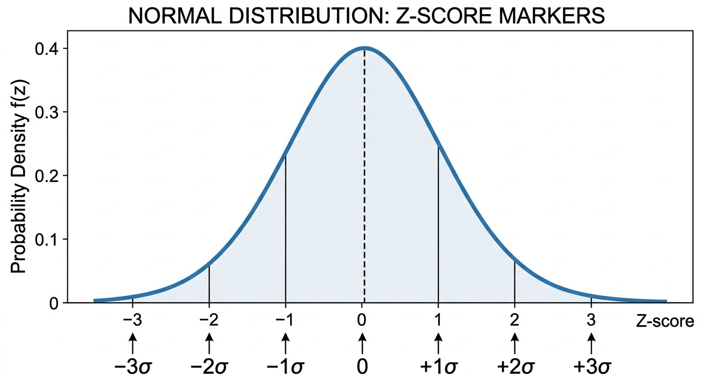
What Is a Z Score?
A z score — also called a standard score or z-value — measures how many standard deviations a data point is from the population mean. Calculated using the formula z = (x − μ) / σ, a z score of 0 means the value equals the mean, positive scores are above average, and negative scores are below average.
The concept dates to the early 20th century, when statisticians needed a way to compare measurements from entirely different scales — a student’s height against their exam score, for instance. By converting both to z scores, any two values become directly comparable, because both are expressed in units of standard deviations from their respective means. According to the NIST Engineering Statistics Handbook, z scores are foundational to the standardization of data and to virtually all parametric hypothesis testing.
What Is the Z Score Formula?
The z score formula standardizes a raw score relative to the population: z = (x − μ) / σ. The numerator measures the distance of x from the mean; dividing by σ expresses that distance in units of standard deviations.
Formula for a Single Data Point
Single Value
z = (x − μ) / σ
Sample Mean
z = (x̄ − μ) / (σ / √n)
| Variable | Symbol | Meaning |
|---|---|---|
| Raw score | x | The individual data point you want to standardize |
| Population mean | μ (mu) | Average of the entire population, not just your sample |
| Population standard deviation | σ (sigma) | Spread of the population data around the mean |
| Z score | z | Number of standard deviations x is from μ |
| Sample mean | x̄ (x-bar) | Mean of your observed sample |
| Sample size | n | Number of observations in your sample |
| Standard error | SE = σ/√n | Standard deviation of the sampling distribution of the mean |
Single Value vs. Sample Mean: Which Formula to Use?
Use the single-value formula when you have one observation from a population with a known mean and standard deviation. Use the sample mean formula when you have computed the mean of n observations and want to test whether that sample mean differs from the population mean. The √n divisor in the denominator comes from the Central Limit Theorem, which establishes that sample means have a standard deviation of σ/√n regardless of the original distribution’s shape, provided n is sufficiently large. This relationship is described in detail in MIT’s Statistics for Applications course materials.
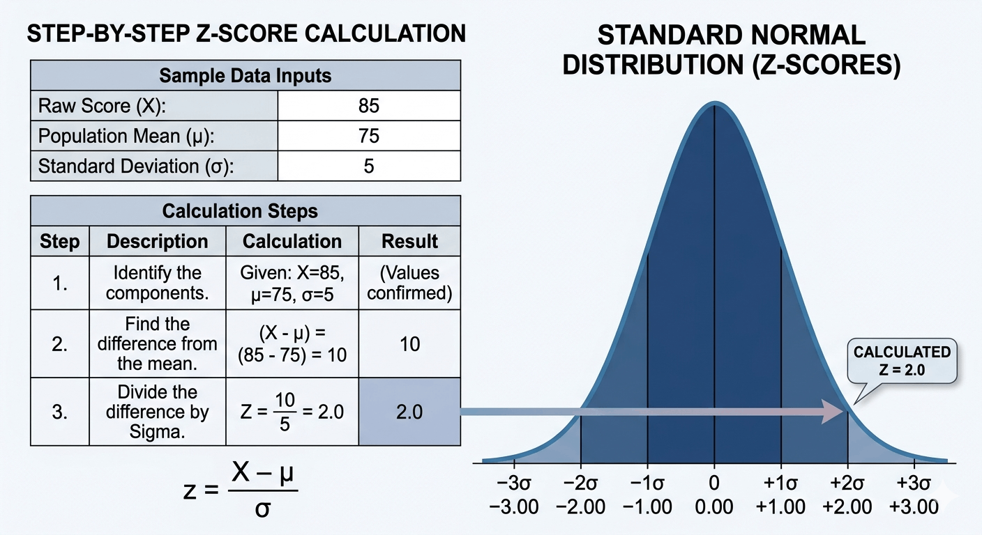
How to Calculate a Z Score: Step-by-Step
Calculating a z score by hand takes exactly four arithmetic steps: subtract the mean, then divide by the standard deviation. The worked example below follows a student’s exam score.
The value you want to standardize. Example: a student scored 85 on an exam.
The average of all values in the full population. Example: class mean = 75.
The spread of the population. Example: σ = 5.
z = (85 − 75) / 5 = 10 / 5 = 2.0
A z score of 2.0 means this student scored 2 standard deviations above the class mean — higher than approximately 97.7% of the class.
Worked Example: Score = 85 | Mean = 75 | σ = 5 → z = (85 − 75) / 5 = 2.0. This places the student at the 97.7th percentile — better than about 97 out of every 100 students in the population.
How to Calculate Z Score in Excel
Excel calculates z scores in a single formula referencing your data range for the mean and standard deviation automatically.
=(A1 - AVERAGE($A$1:$A$100)) / STDEV.P($A$1:$A$100)
Use STDEV.P when your range represents the full population, and STDEV.S when it represents a sample. Drag the formula down to standardize the entire column at once.
How to Read a Z Score: Interpreting Your Results
A z score tells you exactly where a value sits within a normal distribution, expressed as a number of standard deviations from the mean. The interpretation table below maps common z score ranges to their practical meaning.
| Z Score Range | Interpretation | Approx. % of Data Below |
|---|---|---|
| Below −2 | Far below average (outlier territory) | ~2.3% |
| −2 to −1 | Below average | 2.3% – 15.9% |
| −1 to 0 | Slightly below average | 15.9% – 50% |
| 0 | Exactly at the mean | 50% |
| 0 to +1 | Slightly above average | 50% – 84.1% |
| +1 to +2 | Above average | 84.1% – 97.7% |
| Above +2 | Far above average (outlier territory) | ~97.7% |
Negative z scores deserve equal attention — they are not “errors.” A z of −1.5, for instance, appears in roughly 6.7% of normally distributed values, meaning the observation is unusual but not extreme. The symmetry of the standard normal distribution means z = +1.5 and z = −1.5 are equally “far” from the mean in opposite directions.
Z Score Table (Standard Normal Table)
A z score table maps each z score to the cumulative area under the standard normal curve to the left of that point — the left-tail probability. To read it, find the row for the ones and tenths place, then the column for the hundredths place.
Example: z = 1.96 → row 1.9, column 0.06 → probability = 0.9750. This is why 1.96 is the critical value for a 95% two-tailed confidence interval: 97.5% of values fall below z = 1.96, leaving 2.5% in each tail.
| z | .00 | .01 | .02 | .03 | .04 | .05 | .06 | .07 | .08 | .09 |
|---|---|---|---|---|---|---|---|---|---|---|
| 0.0 | .5000 | .5040 | .5080 | .5120 | .5160 | .5199 | .5239 | .5279 | .5319 | .5359 |
| 0.5 | .6915 | .6950 | .6985 | .7019 | .7054 | .7088 | .7123 | .7157 | .7190 | .7224 |
| 1.0 | .8413 | .8438 | .8461 | .8485 | .8508 | .8531 | .8554 | .8577 | .8599 | .8621 |
| 1.5 | .9332 | .9345 | .9357 | .9370 | .9382 | .9394 | .9406 | .9418 | .9429 | .9441 |
| 1.9 | .9713 | .9719 | .9726 | .9732 | .9738 | .9744 | .9750 | .9756 | .9761 | .9767 |
| 2.0 | .9772 | .9778 | .9783 | .9788 | .9793 | .9798 | .9803 | .9808 | .9812 | .9817 |
| 2.5 | .9938 | .9940 | .9941 | .9943 | .9945 | .9946 | .9948 | .9949 | .9951 | .9952 |
| 3.0 | .9987 | .9987 | .9987 | .9988 | .9988 | .9989 | .9989 | .9989 | .9990 | .9990 |
Partial table. View the full z-table for all values from −3.9 to +3.9.
Real-World Examples of Z Scores
Z scores appear in four distinct professional domains. Each example below follows the same formula but demonstrates a different interpretation context.
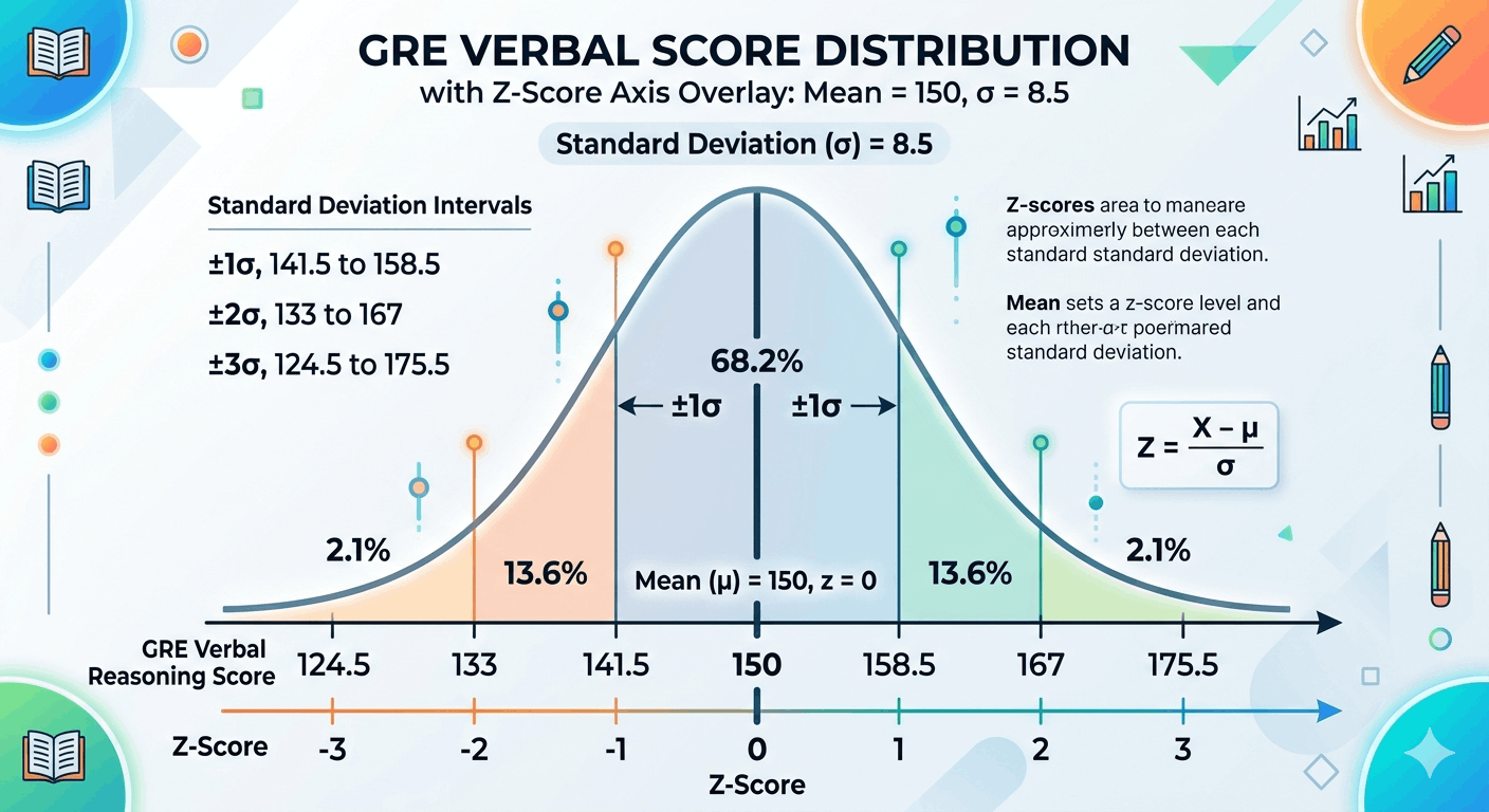
Z Score in Education: Standardized Test Scores
Standardized tests like the SAT and GRE report scaled scores, but z scores reveal the underlying position within the test-taking population. Suppose the verbal GRE has a mean of 150 and σ = 8.5. A score of 162 produces z = (162 − 150) / 8.5 = 1.41, placing the student at approximately the 92nd percentile. College admissions offices use this logic when comparing applicants from different years whose raw scores are not directly comparable. The Educational Testing Service documents the role of standardized scoring in its official score interpretation guides.
Z Score in Finance: The Altman Z-Score
The Altman Z-Score is a multi-variable financial model that uses standardized ratios to predict the probability of corporate bankruptcy within two years. Developed by Edward Altman at New York University in 1968, it combines five financial ratios (working capital/total assets, retained earnings/total assets, and three others) into a single score. Companies scoring above 2.99 fall in the “safe zone,” while those below 1.81 are in the “distress zone.” Credit analysts and equity researchers routinely compute this score before investment decisions. Altman’s original methodology is documented in the Journal of Finance and continues to be cited by risk management practitioners worldwide.
Z Score in Healthcare: Growth Charts
Pediatric growth charts express children’s height and weight as z scores relative to reference populations, allowing clinicians to detect developmental concerns regardless of age. The World Health Organization growth standards define z scores of −2 to +2 as the normal range; values below −2 signal stunting or wasting that may warrant clinical follow-up. A four-year-old in the 3rd percentile for height has a z score of approximately −1.88, which triggers monitoring but not immediate intervention. The WHO publishes the complete methodology at their child growth standards page.
Z Score in Quality Control: Six Sigma
Six Sigma manufacturing targets ±6 standard deviations between the process mean and the nearest specification limit, corresponding to no more than 3.4 defects per million opportunities. In this context, a z score of 6.0 means the nearest defect threshold is six standard deviations from normal operating performance — an extraordinarily tight process. Motorola and General Electric popularized this application in the 1980s and 1990s, and it applies the standard normal distribution directly to manufacturing yield calculations. The American Society for Quality maintains technical resources on Six Sigma methodology.
What Is the Difference Between a Z Score and a T Score?
The key distinction is whether the population standard deviation is known: use a z score when it is, and a t score when it must be estimated from the sample.
| Feature | Z Score | T Score |
|---|---|---|
| Population σ known? | Yes | No — estimated from sample s |
| Sample size | Large (n ≥ 30) | Small (n < 30), or any size with unknown σ |
| Distribution used | Standard normal N(0,1) | Student’s t-distribution with n−1 degrees of freedom |
| Tails | Thinner | Heavier (more probability in extremes for small n) |
| Converges to z when | — | n → ∞ |
As sample size increases, the t-distribution approaches the standard normal. At n = 30, the difference in critical values is already small (t* ≈ 2.045 vs z* = 1.960 for 95% confidence). For most practical applications with n ≥ 30 and a known population SD, z scores give a reliable result. When working with small samples, see the one-sample t-test calculator.
Common Mistakes When Calculating Z Scores
These six errors account for most incorrect z score calculations in student work and applied research. Each one has a straightforward fix.
The formula requires σ (population). Substituting a sample’s s instead produces a biased z score. If population σ is unknown, switch to the t-distribution.
μ is the parameter for the full population, not just your observed data. Confusing the two inflates or deflates the z value.
When working with a sample mean x̄, the denominator must be σ/√n, not σ alone. Omitting √n overstates the evidence by ignoring the smoothing effect of averaging n observations.
Standard z-tables give the left-tail (cumulative) probability Φ(z). For right-tail probability, compute 1 − Φ(z). For a two-tailed test, use 2 × (1 − Φ(|z|)).
A z score of 1.0 is not the 100th percentile. Convert via the CDF: z = 1.0 corresponds to the 84.1st percentile. The z score and the percentile are related, not equal.
The standard normal table only applies when the underlying distribution is approximately normal. For skewed or multimodal data, z scores can be computed but their CDF interpretation is not valid without further transformation.
How to Use This Z Score Calculator
The calculator above has three independent modes. Select the mode that matches your data structure.
Calculator Inputs Explained
The Single Value tab requires three inputs: the raw score x, the population mean μ, and the population standard deviation σ. All three fields are required; leaving any blank will suppress output without generating an error. The Sample Mean tab adds a fourth field for sample size n, which must be a positive integer. The Z to Probability tab takes a z score directly and returns both tail probabilities and the percentile rank without requiring the original data.
Understanding the Output
The summary band at the top shows the four most-requested values: z score, percentile, cumulative probability P(X ≤ x), and a one-line interpretation. The step-by-step panel below shows each arithmetic step in full, so you can verify the calculation by hand or use it as a worked example for coursework. The bell curve diagram shades the left-tail area corresponding to your probability.
When to Use Population vs. Sample Formula
Choose Single Value when your data point came from a population whose mean and standard deviation you already know (or can look up). Choose Sample Mean whenever you are working with the average of a group of observations rather than one individual measurement. The sample size n appears because averaging reduces variability by the factor 1/√n, a property that follows directly from the Central Limit Theorem.
Frequently Asked Questions
A z score (also called a standard score) measures how many standard deviations a data point is from the mean. A z score of 0 means the value equals the mean. A positive z score means above average; a negative z score means below average. Z scores are used in statistics to compare values from different datasets or scales.
The z score formula is: z = (x − μ) / σ, where x is the raw score, μ (mu) is the population mean, and σ (sigma) is the population standard deviation. For a sample mean, the formula becomes z = (x̄ − μ) / (σ / √n), where n is the sample size.
A z score of 1.5 means the data point is 1.5 standard deviations above the population mean. In a normal distribution, approximately 93.3% of values fall below a z score of 1.5. This indicates the data point ranks higher than the large majority of values in the dataset.
Z scores between −2 and +2 are generally within the normal range in a standard distribution, covering about 95% of all data points. A z score above +2 or below −2 indicates an unusually high or low value. Whether a specific z score is “good” depends entirely on context — in testing or finance, a higher score may be better, while in medical screening a very high or low value might indicate a concern.
Yes, a z score can be negative. A negative z score means the raw score falls below the population mean. For example, a z score of −1.2 means the value is 1.2 standard deviations below the mean. Negative z scores are equally valid and common in any normally distributed dataset.
To find probability from a z score, use a z-table (standard normal table) or the “Z to Probability” tab in this calculator. Locate your z score in the table to find the cumulative area under the normal curve to the left of that score. This area equals the left-tail probability (CDF). For a right-tail probability, subtract the table value from 1.
A z score is used when the population standard deviation is known and the sample size is large (n ≥ 30). A t score is used when the population standard deviation is unknown or the sample size is small. Both measure how many standard deviations a value is from the mean, but use different distributions. As n increases, the t-distribution approaches the standard normal.
Z scores are used in standardized testing (SAT, GRE), medical measurements (pediatric growth charts, clinical reference ranges), finance (Altman Z-Score for bankruptcy prediction), quality control (Six Sigma), and research (hypothesis testing and outlier detection). They allow fair comparison of data points from different scales or populations.
To calculate a z score, you need three values: (1) the raw score or data point (x), (2) the population mean (μ), and (3) the population standard deviation (σ). For a sample mean z score, you additionally need the sample size (n) to calculate the standard error σ/√n.
A z score and a percentile both describe a value’s position within a distribution, but they express it differently. A z score gives the number of standard deviations from the mean; a percentile gives the percentage of values that fall at or below that point. The two are related via the CDF: z = 1.0 corresponds to the 84.1st percentile, and z = 1.96 corresponds to the 97.5th percentile.
Related Statistical Calculators
These tools connect directly to z score analysis — each one handles the next step in a typical statistics workflow.