Mean Median Mode Calculator
What Are Mean, Median, and Mode?
Mean, median, and mode are the three measures of central tendency in statistics — each one summarizes an entire dataset with a single representative value. The mean is the arithmetic average. The median is the middle value in a sorted dataset. The mode is the value that appears most often. Together, they answer one core question: where does the center of the data sit?
The term "central tendency" comes from the fact that data in most real-world distributions clusters around a central point. According to the NIST Engineering Statistics Handbook, these three measures are foundational to descriptive statistics and form the basis for all further statistical inference. Choosing the wrong measure — for example, reporting the mean of a skewed salary dataset — can give a misleading picture of reality. That choice matters in data science, economics, public health, and everyday research.
What Is the Mean?
The mean is the sum of all values in a dataset divided by the count of values. It is the most common measure of average and works best when data is roughly symmetric and free of extreme outliers. Its formula is x̄ = Σx / n, where Σx is the total sum and n is the number of values.
Sum = 4 + 8 + 6 + 5 + 3 = 26 | Count = 5 | Mean = 26 ÷ 5 = 5.2
What Is the Median?
The median is the middle value in a dataset after sorting it in ascending order. For an odd number of values, it is the single middle number. For an even number, it is the average of the two middle numbers. The median resists the pull of outliers, making it a better central measure for skewed data.
Even count — Example: Sorted: {2, 4, 6, 8} → Average of 4 and 6 = (4+6)/2 = 5
What Is the Mode?
The mode is the value that appears most frequently in a dataset. It is the only measure of central tendency that works for categorical data (data described by labels rather than numbers, such as colors or survey responses). A dataset can have no mode, one mode, or multiple modes.
Bimodal: {1, 2, 2, 3, 3, 4} → Both 2 and 3 appear twice → Modes = 2 and 3
What Are the Formulas for Mean, Median, and Mode?
Each measure has a distinct formula. The mean uses arithmetic, the median uses position, and the mode uses frequency counting — no formula required.
Mean Formula
x̄ = Σx / n

Where:
Σx = sum of all values
n  = count of values
Median Formula
Odd n:
  Value at (n+1)/2

Even n:
  [x(n/2) + x(n/2+1)] / 2
  (after sorting ascending)
Mode — No Formula
Count frequency of
each value.
The mode = the value
with the highest count.

Can be: none, one,
or multiple modes.
How to Calculate Mean, Median, and Mode Step by Step
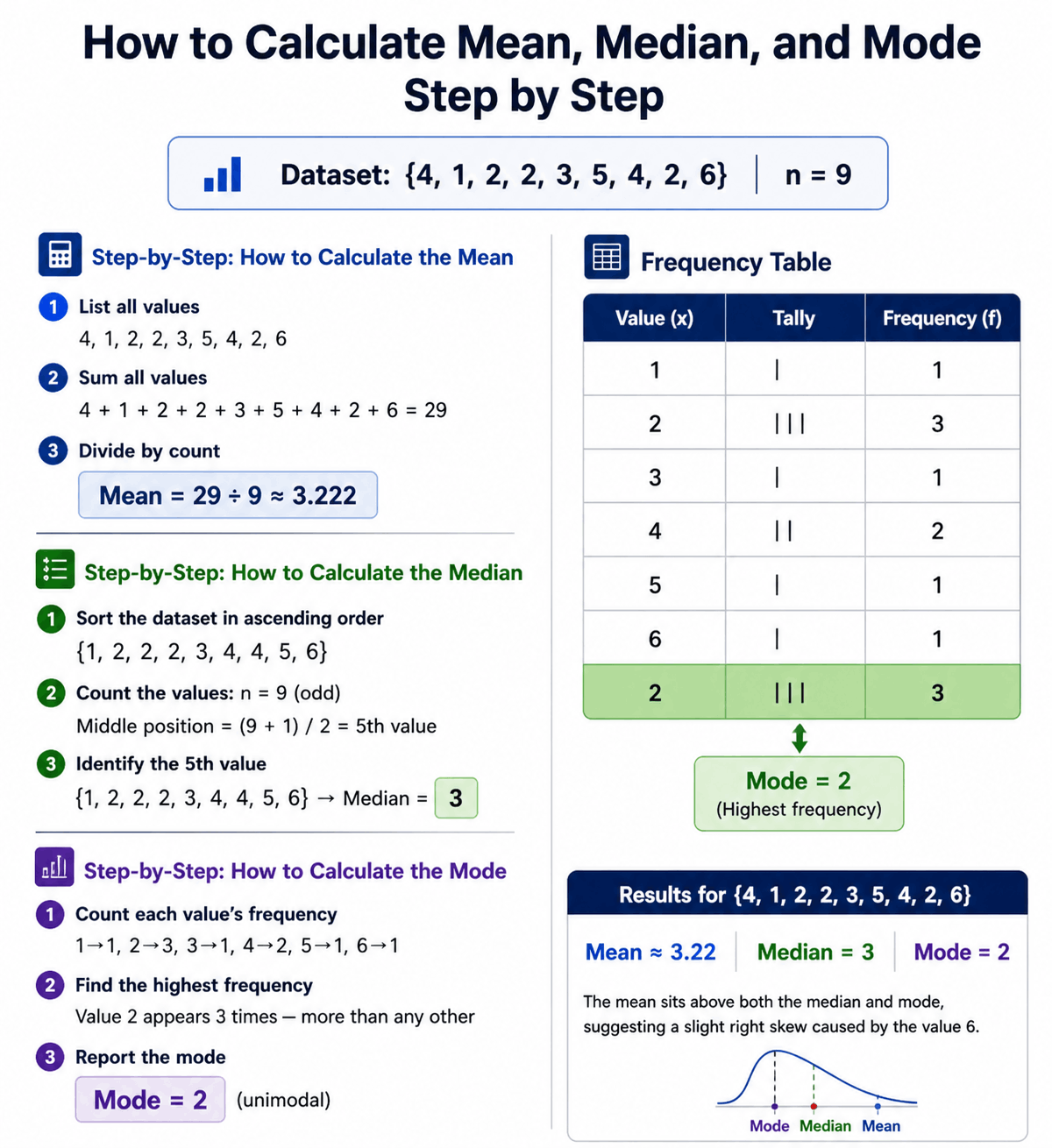
The cleanest approach is to work through all three on the same dataset. Here we use the dataset {4, 1, 2, 2, 3, 5, 4, 2, 6} — nine values.
Dataset: {4, 1, 2, 2, 3, 5, 4, 2, 6} n = 9
Step-by-Step: How to Calculate the Mean
4, 1, 2, 2, 3, 5, 4, 2, 6
4 + 1 + 2 + 2 + 3 + 5 + 4 + 2 + 6 = 29
Mean = 29 ÷ 9 ≈ 3.222
Step-by-Step: How to Calculate the Median
{1, 2, 2, 2, 3, 4, 4, 5, 6}
Middle position = (9 + 1) / 2 = 5th value
{1, 2, 2, 2, 3, 4, 4, 5, 6} → Median = 3
Step-by-Step: How to Calculate the Mode
1→1, 2→3, 3→1, 4→2, 5→1, 6→1
Value 2 appears 3 times — more than any other
Mode = 2 (unimodal)
Results for {4, 1, 2, 2, 3, 5, 4, 2, 6}: Mean ≈ 3.22 | Median = 3 | Mode = 2. The mean sits above both the median and mode, suggesting a slight right skew caused by the value 6.
What Is the Difference Between Mean, Median, and Mode?
The three measures differ in how they are calculated, how they respond to outliers, and which types of data they suit best.
| Feature | Mean | Median | Mode |
|---|---|---|---|
| Best for | Symmetric, continuous data | Skewed data or data with outliers | Categorical or frequency data |
| Affected by outliers? | Yes — significantly | No | No |
| Works with categories? | No | No | Yes |
| Can have multiple values? | No (always one) | No (always one) | Yes (bimodal, multimodal) |
| Real-world example | Average exam score | Median household income | Most common shoe size sold |
| Distribution shape | Mean = Median = Mode (symmetric) | Median between mean and mode (skewed) | Mode at peak (any shape) |
When Should You Use Mean vs. Median vs. Mode?
The right measure depends on the shape of your data, whether outliers exist, and what type of variable you are summarizing. Using the wrong one produces a misleading result.
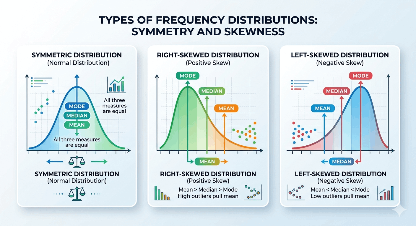
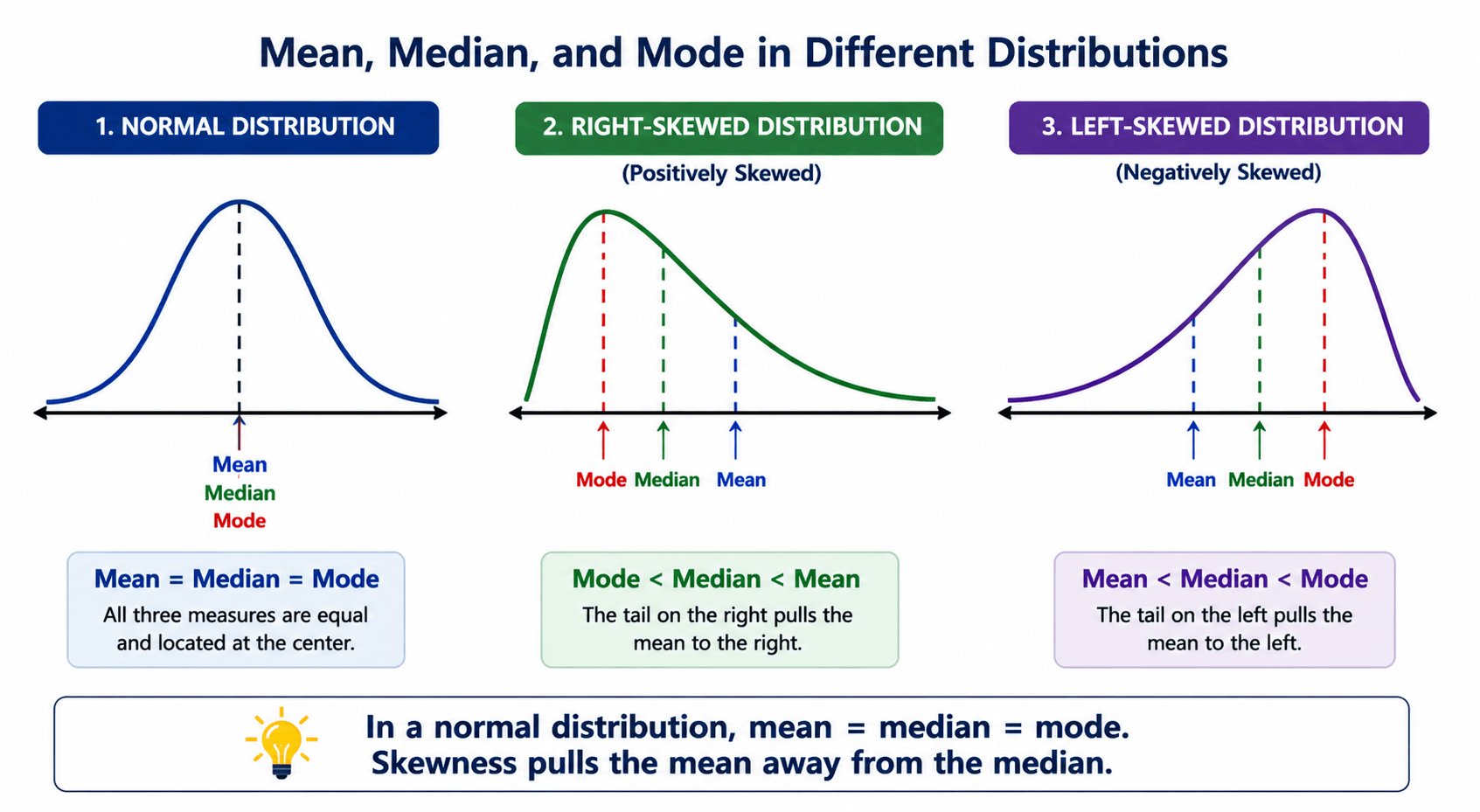
In a perfectly symmetrical, normal distribution, all three measures are equal: mean = median = mode. In right-skewed data (a long tail to the right), the mean is greater than the median, which is greater than the mode. In left-skewed data, the order reverses. This relationship is what gives the comparison of all three measures diagnostic power — if mean and median diverge noticeably, your data is almost certainly skewed.
Worked Examples: Mean, Median, and Mode with Real Data
Example 1: Student Test Scores
Dataset: {72, 85, 90, 85, 60, 95, 72, 85, 78} n = 9
Sum = 72+85+90+85+60+95+72+85+78 = 722 | Mean = 722 ÷ 9 ≈ 80.2
Sorted: {60, 72, 72, 78, 85, 85, 85, 90, 95} | Middle (5th value) = 85
85 appears 3 times (most frequent) | Mode = 85
Interpretation: The mode of 85 shows most students scored in the B range. The mean of 80.2 is pulled down slightly by the outlier score of 60. The median of 85 better represents where the bulk of students scored, making it the more useful summary for this dataset.
Example 2: Salary Data with an Outlier
Dataset: {3200, 3400, 3100, 3300, 3250, 12000} n = 6
Sum = 28,250 | Mean = 28,250 ÷ 6 ≈ $4,708
Sorted: {3100, 3200, 3250, 3300, 3400, 12000} | Middle = (3250+3300)/2 = $3,275
All values appear once | Mode = None
Why this matters: The mean salary of $4,708 is misleading — five of six employees earn between $3,100 and $3,400. One executive earning $12,000 inflates the mean by over $1,400. The median of $3,275 tells the true story. This is exactly why median household income is the standard measure used by the U.S. Census Bureau.
Example 3: No Mode and Bimodal Datasets
Bimodal: Dataset {2, 4, 4, 6, 8, 8} — both 4 and 8 appear twice. Both are modes.
Multimodal: Dataset {1, 1, 2, 2, 3, 3} — three modes: 1, 2, and 3.
Mean, Median, Mode: Complete Formula and Entity Reference
The table below covers every core concept, formula, and use case for measures of central tendency. It is designed for quick reference in exams, data analysis projects, and AI-assisted research.
| Concept | Formula | Plain Explanation | Primary Use Case |
|---|---|---|---|
| Arithmetic Mean | x̄ = Σx / n | Sum of all values divided by their count | Exam averages, temperature data, balanced datasets |
| Median (odd n) | Value at (n+1)/2 | Middle value after ascending sort | Income data, home prices, any skewed distribution |
| Median (even n) | [x(n/2) + x(n/2+1)] / 2 | Average of the two middle values after sorting | Any even-sized dataset requiring a central value |
| Mode | Most frequent value | No arithmetic formula — based purely on frequency counts | Shoe sizes, survey categories, product preferences |
| Range | R = max − min | Distance between the largest and smallest values | Quick spread estimate; used alongside central tendency |
| Population Mean | μ = Σx / N | Mean of an entire population (all possible data points) | Census data, complete population analysis |
| Sample Mean | x̄ = Σx / n | Mean of a subset drawn from a larger population | Survey research, experimental studies, random samples |
| Bimodal | Two equal peak frequencies | Dataset has exactly two modes with equal highest frequency | Detecting two subgroups in a dataset (e.g., two grade clusters) |
| Outlier effect | Affects mean; not median or mode | An extreme value pulls the mean toward it but leaves median unchanged | Deciding whether to report mean or median for skewed data |
| Central Tendency | — | General term for a single value summarizing where data clusters | All descriptive statistics contexts |
How Does Distribution Shape Affect Mean, Median, and Mode?
The relationship between mean, median, and mode changes depending on whether data is symmetric or skewed — and this relationship is itself a diagnostic tool.
In a perfectly symmetric normal distribution, all three measures coincide at the center of the bell curve. As data becomes right-skewed (long tail to the right), the mean gets pulled upward by large values, moving above the median, which in turn sits above the mode. The opposite pattern holds for left-skewed distributions. According to the Khan Academy Statistics review, recognizing this shift is one of the first steps in understanding real-world data distributions.
Right-skewed: Mode < Median < Mean | Example: Incomes, house prices
Left-skewed: Mean < Median < Mode | Example: Age at retirement, survival times
Sources and Further Reading
Authority sources cited in this guide:
- National Institute of Standards and Technology (NIST). Engineering Statistics Handbook — Measures of Location. itl.nist.gov
- U.S. Census Bureau. Income and Poverty in the United States. census.gov
- Khan Academy. Mean, Median, and Mode Review. khanacademy.org
- OpenStax. Introductory Statistics, Chapter 2: Descriptive Statistics. openstax.org
- MIT OpenCourseWare. 18.650 Statistics for Applications. ocw.mit.edu
- Wackerly, Mendenhall & Scheaffer. Mathematical Statistics with Applications, 7th ed. Cengage Learning, 2008.
Related Topics on Statistics Fundamentals
Central tendency connects to a broad network of statistical ideas. These resources build out the full picture from the same foundation.
FAQs: Mean, Median, and Mode
The mean is the arithmetic average of all values, found by dividing the total sum by the count. The median is the middle value when data is sorted in ascending order. The mode is the most frequently occurring value. All three measure central tendency but respond differently to outliers and skewed data — the mean is most sensitive to extreme values, while the median and mode are not.
Add all values together to get the sum, then divide by the number of values. The formula is x̄ = Σx / n. For example, for {4, 8, 6, 5, 3}: sum = 26, count = 5, mean = 26 ÷ 5 = 5.2. This works for any set of numerical values, including decimals and negative numbers.
Sort the data in ascending order, then average the two middle values. For {2, 4, 6, 8} the two middle values are 4 and 6, so the median is (4 + 6) ÷ 2 = 5. For an odd number of values, the median is simply the single middle value — no averaging needed.
A dataset has no mode when every value appears exactly once — no value repeats. For example, {1, 2, 3, 4, 5} has no mode. Some statisticians say in this case "all values are the mode," but this is not standard. A dataset is bimodal if two values share the highest frequency, and multimodal if more than two values do.
Use the median when your data is skewed or contains outliers. A single extreme value can inflate the mean dramatically while leaving the median nearly unchanged. Income data is the classic example: a dataset with five people earning $30,000–$35,000 and one earning $200,000 has a mean of roughly $63,000 — far above what any of the five typical earners actually makes. The median of around $32,500 is far more representative.
Yes — in a perfectly symmetric distribution, mean and median are equal. This is a defining property of the normal (bell curve) distribution. In skewed distributions they diverge: right-skewed data pulls the mean above the median, while left-skewed data pushes the mean below it. If mean and median are very close, your data is likely approximately symmetric.
Mean: calculating class averages, tracking daily temperatures, measuring manufacturing tolerances. Median: reporting household income (U.S. Census Bureau standard), housing price reports, clinical trial outcomes. Mode: finding the most common blood type in a patient group, identifying the best-selling product size, analyzing the most frequent response in a customer satisfaction survey.
In a normal (bell-shaped) distribution, mean = median = mode. All three coincide at the peak of the curve. This equality is a key reason the normal distribution is so central to statistics — it means any of the three measures accurately locates the center. As data deviates from normality, the three measures separate, and that separation itself signals the nature of the deviation.