Pearson r Critical Value Calculator
What Is a Pearson Correlation Critical Value?
The Pearson correlation coefficient r measures the strength and direction of the linear relationship between two continuous variables. It takes values from −1 to +1. But a non-zero r computed from a sample does not automatically mean a real relationship exists in the population — it could have appeared by chance.
The critical value rcrit is the threshold that separates a sample r that is plausibly due to chance from one that is too large to attribute to chance at the chosen α level. The decision rule is direct: if |r| ≥ rcrit, reject H₀; if |r| < rcrit, do not reject H₀.
Key distinction: r is what you calculate; rcrit is what you look up. Statistical significance means |r| ≥ rcrit. It does not tell you whether the relationship is practically meaningful. A correlation of r = 0.20 can be significant with n = 200, yet explain only 4% of variance.
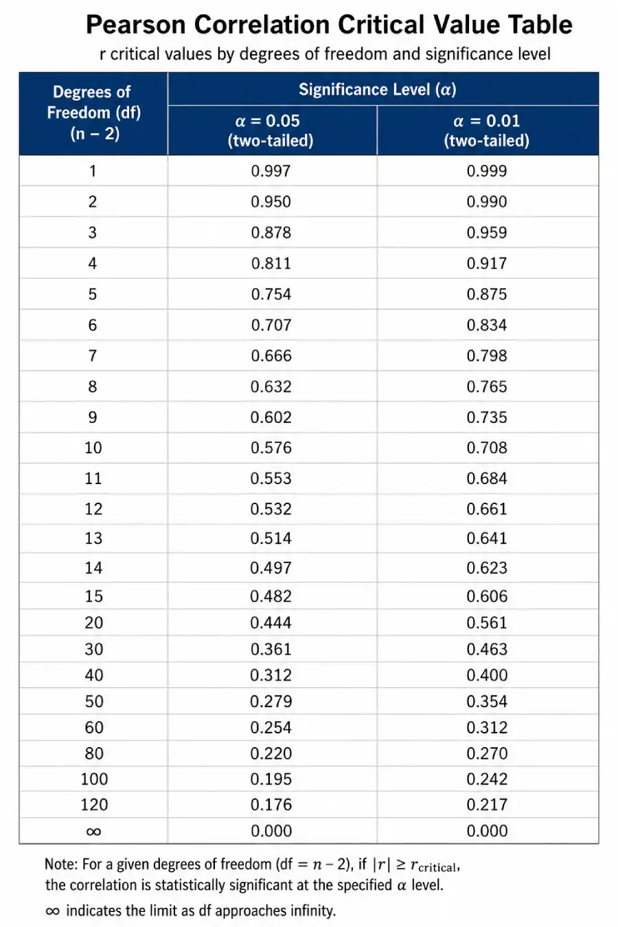
Pearson Correlation Critical Value Table (Core Reference)
All values below are rcrit — the minimum |r| for statistical significance. Select the tab matching your test direction and α level. Click any cell to highlight and load it into the calculator above.
df = n − 2. Reject H₀ if |r| ≥ rcrit. Values sourced from Cohen, J., Cohen, P., West, S. G., & Aiken, L. S. (2003) and validated against the t-distribution conversion t = r√(n−2)/√(1−r²). n = sample size (number of paired observations).
How Pearson Correlation Hypothesis Testing Works
Testing the significance of a Pearson r follows a structured procedure. Each step below corresponds to a specific statistical decision.
Step 1 — State Hypotheses
The null hypothesis is always H₀: ρ = 0 (no linear correlation exists in the population). The alternative depends on your test direction: H₁: ρ ≠ 0 (two-tailed, standard), H₁: ρ > 0 (one-tailed, positive), or H₁: ρ < 0 (one-tailed, negative). Set your α level before collecting data, typically α = 0.05.
Step 2 — Compute Pearson r
Calculate r from paired data (x, y):
r = +1: perfect positive linear relationship. r = 0: no linear relationship. r = −1: perfect negative linear relationship. Most statistical software (R, Python, SPSS, Excel) computes r directly.
Step 3 — Find Sample Size (n) and df = n − 2
n is the number of paired (x, y) observations. Degrees of freedom df = n − 2. Two degrees are lost because the test estimates both the sample mean of x and the sample mean of y. With n = 30, df = 28; with n = 100, df = 98.
Step 4 — Look Up r Critical
Find the row in the table above that matches your df. Read across to the column for your chosen α and test direction. That cell gives rcrit. If your exact df is not listed, use the next smaller df (the conservative choice) or interpolate.
Step 5 — Compare |r| vs r Critical
If |r| < rcrit → Fail to reject H₀ → Not statistically significant
Step 6 — Report the Result
Report r, n (or df), the test direction, α, and your conclusion. APA format: r(18) = .52, p < .05 (two-tailed). Reporting r² alongside r (the coefficient of determination) adds context for practical significance: r = 0.52 means r² = .27, so 27% of variance in y is linearly associated with x.
Two-Tailed vs One-Tailed Correlation Test
The test direction determines which column in the table to use and directly affects the critical value. The choice must be made based on your hypothesis — not after examining the data.
Two-Tailed — Standard Choice
Detects a correlation in either direction (r could be positive or negative). Used in most academic research where no directional prediction was made beforehand. The critical region is split between both tails of the distribution.
One-Tailed — Directional Hypothesis
Used only when prior theory or research justifies predicting a specific direction before data collection. The one-tailed critical value is smaller, providing more power — but misapplying it inflates Type I error.
Worked Example: Testing Pearson r Step by Step
Scenario: An education researcher collects data on weekly study hours (x) and exam scores (y) from 25 students. She computes r = 0.43 and wants to know whether this correlation is statistically significant at α = 0.05 (two-tailed).
Solution — Step by Step
| Step | Action | Result |
|---|---|---|
| 1 | State H₀ and H₁ | H₀: ρ = 0; H₁: ρ ≠ 0; α = 0.05, two-tailed |
| 2 | Record computed r | r = 0.43 |
| 3 | Compute df | df = n − 2 = 25 − 2 = 23 |
| 4 | Look up rcrit | df=23, α=0.05, two-tailed → rcrit = 0.396 |
| 5 | Compare |r| vs rcrit | |0.43| = 0.43 > 0.396 → Reject H₀ |
Interpretation
With r(23) = 0.43, p < 0.05 (two-tailed), the correlation between weekly study hours and exam scores is statistically significant. r² = 0.185, meaning approximately 18.5% of the variance in exam scores is linearly associated with study hours. The remaining 81.5% of variance is attributed to other factors not in this analysis.
Visual Interpretation: r vs r Critical
Two factors determine whether a correlation reaches significance: the size of r and the sample size n. The table below illustrates how the same r value can be significant in a large sample but not in a small one.
| Computed r | n = 10 (rcrit = 0.632) | n = 30 (rcrit = 0.361) | n = 100 (rcrit = 0.197) |
|---|---|---|---|
| 0.20 | Not sig. | Not sig. | Sig. ✓ |
| 0.40 | Not sig. | Sig. ✓ | Sig. ✓ |
| 0.65 | Sig. ✓ | Sig. ✓ | Sig. ✓ |
| 0.90 | Sig. ✓ | Sig. ✓ | Sig. ✓ |
All comparisons use two-tailed α = 0.05. rcrit values taken from the table above.
Why Sample Size Matters
As n grows, df = n − 2 increases and rcrit falls. A larger sample gives more statistical power — the ability to detect a real correlation that exists in the population. This is why a study with n = 200 can report r = 0.15 as significant while a study with n = 15 needs r ≥ 0.514 to reach the same threshold.
This also underscores a well-established statistical point: significance is not the same as importance. An r = 0.15 that is significant with n = 200 accounts for only r² = 0.023, or 2.3% of variance. Reporting effect sizes alongside p-values gives a more complete picture.
Interpreting Pearson r: Strength, Direction, and Significance
Three separate questions apply to any Pearson r: Is it statistically significant? How strong is it? What direction is it? The table answers the first question only.
These thresholds follow Cohen's (1988) guidelines for behavioral research. Other fields use different benchmarks. In psychometrics, r > 0.70 is often required for test reliability. In physics, r > 0.99 may be expected. Context always determines what constitutes a practically meaningful correlation.
Statistical Significance vs Practical Significance
The r critical table only determines statistical significance. It answers: Is this correlation larger than chance alone predicts? It does not answer: Is this correlation large enough to matter in practice? For that, researchers report r² (the proportion of shared variance) alongside the significance test. Both pieces of information are needed for a complete interpretation. This distinction is discussed in detail in the standard deviation and variance context on Statistics Fundamentals.
Applied Examples Across Research Fields
The following examples show how the critical value table applies to realistic research questions. Each uses a different sample size to illustrate how n affects the significance threshold.
Psychology: Stress and Academic Performance
A researcher measures perceived stress (PSS scores) and GPA for n = 40 undergraduates and finds r = −0.32. With df = 38, rcrit = 0.312 (α = 0.05, two-tailed). Since |−0.32| = 0.32 > 0.312, the correlation is significant. r² = 0.10: stress accounts for 10% of GPA variance in this sample.
Education: Study Time and Exam Grades
A study with n = 15 students finds r = 0.50 between hours studied and exam score. With df = 13, rcrit = 0.514 (α = 0.05, two-tailed). Since 0.50 < 0.514, the result does not reach significance. The same r = 0.50 with n = 30 would be significant (rcrit = 0.361).
Business: Ad Spend and Revenue
Monthly advertising expenditure and sales revenue over n = 50 periods yields r = 0.61. With df = 48, rcrit = 0.279 (α = 0.05, two-tailed). The correlation is significant; r² = 0.37 indicates advertising expenditure and revenue share 37% of variance. This does not establish causation.
Health Research: Physical Activity and BMI
A health survey with n = 100 participants produces r = −0.21 between weekly exercise (hours) and BMI. With df = 98, rcrit = 0.197 (α = 0.05, two-tailed). The correlation is significant. However, r² = 0.044 indicates only 4.4% of BMI variance is linearly associated with exercise frequency in this data.
r vs r Critical Decision Rule
The core decision rule for Pearson correlation significance testing applies regardless of which α level or test direction you choose:
If |r| ≥ rcrit → Reject H₀ → Correlation is statistically significant at α
If |r| < rcrit → Fail to reject H₀ → Insufficient evidence of correlation at α
The alternative approach uses the t-statistic directly: convert r to t = r√(n−2)/√(1−r²) and compare against the t-distribution critical value with df = n − 2 at the same α. Both methods produce identical decisions. The r critical table is the more direct route when the only goal is a significance decision for Pearson r.
Symbol and Concept Glossary
The table below defines every symbol involved in the Pearson correlation significance test. It also notes the most common misinterpretation for each.
| Symbol | Name | Definition | Common Error |
|---|---|---|---|
| r | Pearson correlation coefficient | Sample measure of linear relationship; −1 to +1 | Assuming r implies causation |
| ρ | Population correlation | True correlation in the full population; tested via H₀: ρ = 0 | Treating r as if it were ρ |
| rcrit | Critical value | Minimum |r| for significance at chosen α and df | Using n directly instead of df = n − 2 |
| n | Sample size | Number of paired (x, y) observations | Counting individuals instead of pairs |
| df | Degrees of freedom | df = n − 2; governs which row to look up | Using df = n − 1 or df = n |
| α | Significance level | Probability of a Type I error; selects table column | Setting α after examining the data |
| r² | Coefficient of determination | Proportion of variance in y linearly associated with x | Confusing with explained causation |
| t | Test statistic (alternative) | t = r√(n−2)/√(1−r²); equivalent to using rcrit | Using wrong df in t-table lookup |
Quick Lookup: Most Commonly Used r Critical Values
These are the most frequently referenced values for two-tailed tests at α = 0.05 and α = 0.01 — the standard levels used in most published research.
| n | df | rcrit (α=0.05, 2-tail) | rcrit (α=0.01, 2-tail) |
|---|---|---|---|
| 5 | 3 | 0.878 | 0.959 |
| 10 | 8 | 0.632 | 0.765 |
| 20 | 18 | 0.444 | 0.561 |
| 30 | 28 | 0.361 | 0.463 |
| 50 | 48 | 0.279 | 0.361 |
| 100 | 98 | 0.197 | 0.256 |
Assumptions of the Pearson Correlation Test
The r critical value table produces valid significance decisions only when the following conditions are met. Violations do not always invalidate results but should be checked before interpreting output.
Linearity
Pearson r measures only linear association. A non-linear relationship (curved, U-shaped) can produce r ≈ 0 even when a strong relationship exists. Always plot a scatterplot first.
Continuous Variables
Both x and y should be measured on interval or ratio scales. For ordinal data, Spearman's ρ is more appropriate. For binary outcomes, point-biserial correlation applies instead.
Bivariate Normality
For valid significance testing, the joint distribution of (x, y) should be approximately bivariate normal. With larger n (≥ 30), the test is fairly robust to this assumption due to the Central Limit Theorem.
Independence
Each (x, y) pair should come from an independent observation. Repeated measures, time-series data, or clustered observations violate this assumption and require different methods.
No Influential Outliers
A single outlier can substantially inflate or deflate r. Before reporting results, check for outliers in the scatterplot and, where appropriate, report r with and without influential points to assess stability.
Frequently Asked Questions About the Pearson Correlation Table
What is a Pearson correlation critical value?
A Pearson correlation critical value (rcrit) is the minimum absolute value of r needed to reject the null hypothesis H₀: ρ = 0 at a given significance level. It depends on degrees of freedom df = n − 2 and whether the test is one- or two-tailed.
How do you find degrees of freedom for correlation?
df = n − 2, where n is the number of paired observations. For example, if you measured height and weight for 30 people, n = 30 and df = 28. Use df to find the row in the table, not n directly.
What is the difference between r and r critical?
r is the correlation coefficient you compute from your sample data. rcrit is a threshold from the table that represents the minimum correlation attributable to chance at a given α. You compare |r| against rcrit to make a significance decision.
What happens if r is less than r critical?
If |r| < rcrit, you fail to reject H₀: ρ = 0. The observed correlation is not large enough to rule out sampling variation as the explanation. This does not prove the correlation is zero in the population — it means this sample does not provide sufficient evidence of one.
Is Pearson correlation affected by sample size?
Yes. The critical value rcrit decreases as n increases, making it easier to achieve statistical significance with larger samples. With n = 10, r must be at least 0.632 (α = 0.05, two-tailed). With n = 100, r only needs to reach 0.197. This is why large-sample correlations can be statistically significant even when r² is very small.
How is the Pearson r test related to linear regression?
In simple linear regression, the significance test for the slope β₁ is mathematically equivalent to the significance test for Pearson r. Both produce the same t-statistic with df = n − 2 and the same p-value. r² in correlation equals the R² in the regression output. See the Statistics Fundamentals regression guide for details.
When should I use Pearson vs Spearman correlation?
Use Pearson r when both variables are continuous and the relationship appears linear in a scatterplot, with no severe outliers. Use Spearman's ρ when variables are ordinal, the relationship is monotonic but not linear, or substantial outliers are present. The two tests use separate critical value tables.
What if my df is not in the table?
If your exact df is absent, use the next smaller df listed — this is the conservative approach. Alternatively, interpolate between adjacent rows. For precise p-values at any df, use the t-statistic conversion: t = r√(n−2)/√(1−r²), then look up the resulting t in a t-distribution table with df = n − 2.
Sources & Further Reading
The critical values in this table are derived from the t-distribution with df = n − 2, using the equivalence rcrit = tcrit / √(tcrit² + df). Values are validated against the following standard references:
Cohen, J., Cohen, P., West, S. G., & Aiken, L. S. (2003). Applied Multiple Regression/Correlation Analysis for the Behavioral Sciences (3rd ed.). Lawrence Erlbaum. Appendix B — Pearson r critical value tables and effect size conventions widely used in behavioral research. doi:10.4324/9780203774441
Penn State STAT 501: Regression Methods. Lesson 1: Simple Linear Regression — Correlation. Pennsylvania State University. online.stat.psu.edu/stat501/lesson/1/1.9 — Open-access course notes covering the relationship between the Pearson r test statistic and the t-distribution.
NIST/SEMATECH e-Handbook of Statistical Methods (2013). Section 1.3.6.7: Critical Values of the Correlation Coefficient. National Institute of Standards and Technology. itl.nist.gov — U.S. government statistical reference covering correlation testing methodology.
UCLA Statistical Methods and Data Analytics. What is the Pearson Correlation Coefficient? University of California, Los Angeles. stats.oarc.ucla.edu — Detailed explanation of the Pearson r formula, assumptions, and interpretation with worked examples.
Yale University Department of Statistics (2025). STAT 101: Correlation and Regression. Yale University. stat.yale.edu — Yale course materials on the Pearson correlation coefficient, linearity assumption, and hypothesis testing framework.
Related Statistical Tables & Resources
Understanding What the Pearson r Table Tells You
Why rcrit Decreases as n Increases
Larger samples yield more precise estimates of the population correlation ρ. With more data, smaller deviations from zero become detectable. A sample of 200 can reliably distinguish ρ = 0.14 from zero; a sample of 10 cannot. The rcrit table encodes this precision-to-sample-size relationship.
Relationship Between r Critical and t Critical
The Pearson r significance test and the one-sample t-test share the same underlying distribution. Converting r to t (using t = r√(df)/√(1−r²)) and comparing against the t critical value produces an identical decision to comparing |r| against rcrit. The two approaches are mathematically equivalent at the same df and α.
Why Correlation Does Not Imply Causation
A statistically significant r confirms that a linear relationship is unlikely to be due to chance sampling — it says nothing about why the relationship exists. Confounding variables, reverse causation, or coincidence can all produce a significant r. Establishing causation requires experimental design, not correlation alone. See the study design section for details on controlled experiments.