What Are Types of Data?
Every dataset is made up of variables, and every variable has a type. That type is not a formality — it is the first decision in any analysis. Apply the wrong statistical test to the wrong data type, and your results are meaningless no matter how carefully the rest of the math is done.
The NIST/SEMATECH Engineering Statistics Handbook defines measurement scales as the foundation of statistical analysis, noting that "the distinction between types of data is fundamental to the appropriate choice of statistical methods." Understanding data types also builds the vocabulary shared across research disciplines: a psychologist and an epidemiologist use the same framework to describe their variables, even when the variables themselves differ entirely.
At Statistics Fundamentals, this classification framework connects directly to every other topic on the site. The descriptive statistics you can compute depend on it. The data visualizations appropriate for your data depend on it. And the hypothesis tests available to you depend on it.
Why Data Classification Matters
Consider three variables from a student dataset: student ID number, grade level (Freshman/Sophomore/Junior/Senior), and GPA. All three contain numbers or labels, but they require completely different treatment:
- Student ID is a nominal label — averaging IDs produces a nonsensical number
- Grade level is ordinal — Freshman < Sophomore < Junior < Senior, but the gaps are not measurably equal
- GPA is ratio scale — you can calculate a meaningful average, and a 4.0 is genuinely twice a 2.0
Researchers at Penn State's Department of Statistics note in their online curriculum that choosing the wrong analysis based on a misclassified variable is one of the most common errors in introductory statistical work (Penn State STAT 500).
- Qualitative (Categorical): Describes characteristics or group membership — blood type, color, country
- Quantitative (Numerical): Represents counts or measurements — height, income, test scores
- Discrete: Countable whole numbers — number of children, defects per batch
- Continuous: Any value in a range — temperature, weight, distance
- Nominal: Categories without natural order — gender, product category
- Ordinal: Ranked categories with unequal gaps — satisfaction ratings, education level
- Interval: Equal gaps, no true zero — Celsius temperature, calendar years
- Ratio: Equal gaps with true zero — weight, age, income
The Two Main Types of Data: Qualitative vs. Quantitative
Every variable in a dataset starts with one fundamental question: is it a category or a number? This distinction separates qualitative from quantitative data and determines the entire analytical pathway that follows.
Qualitative Data (Categorical Data)
Describes groups, labels, or characteristics — not amounts
Qualitative data places observations into named groups. You cannot add, subtract, or calculate an average from it in a meaningful way. Analysis focuses on counting frequencies, comparing proportions, and testing for associations between groups.
Qualitative data answers the question "what kind?" It describes membership in a group rather than how much of something exists. A patient's diagnosis, a customer's preferred payment method, the name of a city — these are all qualitative. Note that qualitative data can contain numbers as labels (like ZIP codes or phone numbers) without those numbers being mathematically meaningful.
Quantitative Data (Numerical Data)
Represents measurable amounts where arithmetic makes sense
Quantitative data records actual quantities. You can calculate means, compute differences, and perform the full range of statistical operations. The values carry genuine numeric meaning — the difference between 10 and 20 is the same as the difference between 90 and 100.
Quantitative data answers "how many?" or "how much?" The key test is whether arithmetic operations produce meaningful results. The mean of 20 exam scores tells you something real about classroom performance. The "mean" of 20 ZIP codes tells you nothing.
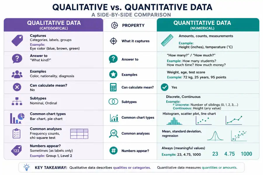
Qualitative vs. Quantitative Data: Comparison
| Property | Qualitative Data | Quantitative Data |
|---|---|---|
| What it captures | Categories, labels, groups | Amounts, counts, measurements |
| Answer to | "What kind?" | "How many?" / "How much?" |
| Examples | Color, nationality, diagnosis | Weight, age, test score |
| Can calculate mean? | No | Yes |
| Subtypes | Nominal, Ordinal | Discrete, Continuous |
| Common chart types | Bar chart, pie chart | Histogram, scatter plot, line chart |
| Common analyses | Frequency counts, chi-square test | Mean, standard deviation, regression |
| Numbers appear? | Sometimes (as labels only) | Always (meaningful values) |
Discrete vs. Continuous Data
Within quantitative data, there is another split that affects both visualization and analysis: whether values are countable whole numbers (discrete) or can take any value in a range (continuous). This distinction determines whether a bar chart or a histogram is more appropriate, and whether a Poisson model or a normal model fits your data better.
Discrete Data
Discrete data can only take specific, countable values. Usually these are non-negative integers, though the defining characteristic is that you cannot have a meaningful value between two adjacent possible values. You can have 3 children or 4, but not 3.6 children. You can receive 0 complaints or 1 complaint, but the gap between those two values is absolute.
Countable values with no meaningful values in between
Each observation is a whole unit. The question to ask: "Can I always insert another possible value between any two values in my dataset?" If the answer is no, the data is discrete.
Continuous Data
Continuous data can take any value within a range, including every fraction and decimal. Between any two possible measurements, there is always another possible value. Height, temperature, time, and weight are all continuous because a person could theoretically be 170.4, 170.41, or 170.413 cm tall — there is no natural stopping point for precision.
Measurable values where any decimal is theoretically possible
Continuous data can always be subdivided further in theory, limited only by measurement instrument precision. The gaps between values are not fixed — they depend on how precisely you measure.
Common Classification Mistakes
Age measured to the day or year is continuous ratio data. But when a study records age as "under 30 / 30–50 / over 50," it becomes ordinal categorical data. The same underlying phenomenon can yield different data types depending on how the measurement is recorded. Always check the measurement instrument and recording method, not just the variable name.
Star ratings (1–5 stars) cause frequent confusion. Technically they are ordinal qualitative data — the gaps between stars are not proven to be equal in the rater's mind. In practice, many researchers treat Likert scale responses as interval data for analysis convenience, but this is an assumption that requires justification. The American Psychological Association's measurement guidelines recommend explicitly stating this assumption when used.
| Feature | Discrete Data | Continuous Data |
|---|---|---|
| Values | Specific, countable whole units | Any value in a range |
| Values in between | No (gaps are absolute) | Yes (infinite precision possible) |
| Test question | "Can I count exact whole numbers?" | "Can I measure to a decimal?" |
| Common distribution | Binomial, Poisson | Normal, Uniform, Exponential |
| Best chart | Bar chart | Histogram, density plot |
| Examples | Children per household, defects | Height, reaction time, temperature |
Levels of Measurement: Nominal, Ordinal, Interval, Ratio
The most precise classification framework in statistics comes from psychologist Stanley Smith Stevens, who introduced the four measurement scales in 1946 in the journal Science. His framework, now a core part of research methods education worldwide, defines nominal, ordinal, interval, and ratio scales based on the mathematical properties each scale possesses. The framework is taught in virtually every undergraduate statistics curriculum, including courses at MIT and Stanford.
Think of the four scales as a ladder of mathematical power. Each rung adds a new property to the ones below it, unlocking additional operations and analyses.
The Four Measurement Scales — From Least to Most Mathematically Powerful
Nominal — Labels Only
Categories with no natural order. You can count frequency but cannot rank, add, or compute averages. Operations: = and ≠ only.
Ordinal — Ranked Order (Unequal Gaps)
Categories that can be ranked, but the gaps between ranks are not necessarily equal. You can say "more than" or "less than" but not "how much more." Operations: =, ≠, >, <.
Interval — Equal Gaps (No True Zero)
Measured values with equal, meaningful intervals between points — but no true zero. Differences are meaningful; ratios are not. You cannot say 20°C is "twice as hot" as 10°C. Operations: =, ≠, >, <, +, −.
Ratio — Equal Gaps + True Zero
All properties of interval scale, plus a meaningful zero that represents complete absence. Ratios are valid: 100 kg is genuinely twice 50 kg. The full range of statistical operations applies. Operations: =, ≠, >, <, +, −, ×, ÷.
Nominal Data
Nominal data puts observations into named boxes with no implied ranking between them. The word "nominal" comes from the Latin nomen (name) — these are genuinely just names or labels. Changing the order in which you list nominal categories does not change any information about the data.
Unordered categories — names and labels only
There is no sense in which one nominal category is "higher" or "more" than another. You cannot rank blood type A above blood type B; they are simply different groups.
The appropriate statistics for nominal data are frequency counts, proportions, and the mode. The appropriate test for comparing two groups' nominal distributions is the chi-square test. You cannot calculate a mean for nominal data — "the average blood type is 1.73" means nothing.
Ordinal Data
Ordinal data adds rank order to the nominal properties. You know that one category is "higher" than another, but you cannot measure how much higher. The distance between Rank 1 and Rank 2 is not necessarily the same as the distance between Rank 2 and Rank 3.
Ranked categories — order matters, gaps do not
The position in the ranking carries information, but the size of the gap between positions does not. A customer who gives a product 5 stars is more satisfied than one who gives 3 stars, but you cannot claim they are exactly "2 units" more satisfied.
For ordinal data, median and rank-based statistics are appropriate. You should not calculate a mean for ordinal data, though in practice many researchers do so for Likert scales and note the assumption explicitly. Non-parametric tests like the Mann-Whitney U test or Spearman rank correlation apply directly to ordinal data.
Interval Data
Interval data is where arithmetic genuinely begins to apply. The gaps between values are equal and measurable, so differences carry real meaning. The complication is the lack of a true zero. In the Celsius scale, 0°C was defined arbitrarily as the freezing point of water — it does not mean "no temperature exists." This is why you cannot say 20°C is twice as hot as 10°C.
Equal gaps between values — but zero is arbitrary
Differences are meaningful and comparable. Ratios are not. The scale has no natural origin; its zero point was chosen by convention rather than representing the true absence of the thing being measured.
Before claiming ratio statements, apply this test: does zero mean complete absence? For temperature in Celsius, 0°C does not mean "no temperature" — it is just the freezing point of water. You can say the temperature rose by 10 degrees, but not that 20°C is twice as warm as 10°C. Convert to Kelvin (which has a true absolute zero), and ratio statements become valid.
Ratio Data
Ratio data has all the properties of interval data, with one addition: a true, meaningful zero that represents the complete absence of the measured quantity. Zero kilograms means no weight. Zero income means no income. Zero reaction time is physically impossible, which confirms reaction time is ratio scale. Because the zero is real, you can make valid ratio comparisons.
All interval properties plus a true, meaningful zero
The most mathematically powerful data type. Every arithmetic operation is valid. A value of zero means the measured quantity is completely absent, not just a convention or reference point.
Most physical measurements — weight, height, time elapsed, distance, counts of events — are ratio scale. This is the richest data type because the complete suite of statistical operations applies: mean, standard deviation, ratios, percentages, and all parametric tests.
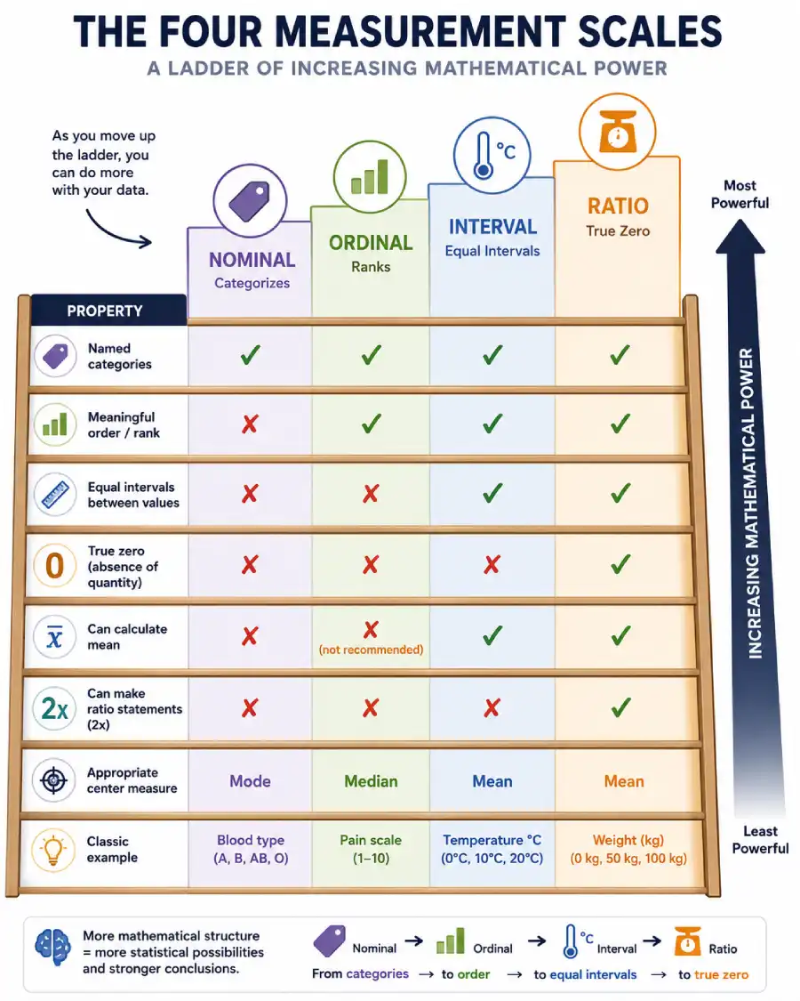
NOIR Comparison: All Four Scales Side by Side
| Property | Nominal | Ordinal | Interval | Ratio |
|---|---|---|---|---|
| Named categories | ✓ | ✓ | ✓ | ✓ |
| Meaningful order / rank | ✗ | ✓ | ✓ | ✓ |
| Equal intervals between values | ✗ | ✗ | ✓ | ✓ |
| True zero (absence of quantity) | ✗ | ✗ | ✗ | ✓ |
| Can calculate mean | ✗ | ✗ (not recommended) | ✓ | ✓ |
| Can make ratio statements (2x) | ✗ | ✗ | ✗ | ✓ |
| Appropriate center measure | Mode | Median | Mean | Mean |
| Classic example | Blood type | Pain scale | Temperature °C | Weight (kg) |
Interactive Data Type Classifier
Answer the questions below to identify the correct data type for any variable in your dataset. The classifier walks through the same decision logic used in statistical textbooks at institutions like Penn State and Harvard's Department of Statistics.
🔬 Data Type Classifier — What Kind of Data Do You Have?
Answer each question about your variable. The tool will identify the data type and suggest appropriate statistical methods.
Primary vs. Secondary Data
Separate from the nominal/ordinal/interval/ratio classification, researchers also categorize data by its origin: was it collected firsthand for this study, or does it come from an existing source? This distinction matters for research validity, cost, and the types of conclusions you can draw.
Primary Data
Primary data is collected directly by the researcher for the specific research question at hand. The collector controls the measurement instrument, the sampling process, and the variables recorded.
First-hand data collected for your specific study
You define exactly what gets measured, how, and from whom. Primary data is tailored precisely to your research question, but it costs time and money to collect.
Secondary Data
Secondary data was collected by someone else for a different original purpose. The researcher reuses it for a new analysis. Secondary data is faster and cheaper to access, but it may not perfectly match the research question.
Existing data reused from a different original study or source
Government agencies, academic institutions, and businesses collect enormous datasets. Researchers can access these for new analyses without the cost of original data collection.
The U.S. Census Bureau's data.census.gov and the World Health Organization's Global Health Observatory are among the most widely used secondary data sources in academic research. A researcher studying income inequality does not need to survey millions of households — that data already exists.
| Factor | Primary Data | Secondary Data |
|---|---|---|
| Who collected it | The researcher themselves | Someone else, for another purpose |
| Cost | High (surveys, labs, field work) | Low to free (often publicly available) |
| Time to obtain | Slow (months to years) | Fast (often immediate access) |
| Tailored to question? | Yes — fully customizable | Rarely — may require adaptation |
| Reliability | High (you control quality) | Variable (depends on original source) |
| Examples | Clinical trials, surveys, experiments | Census data, WHO statistics, academic datasets |
Structured vs. Unstructured Data
Modern data science adds a third classification dimension that traditional statistics did not need: whether data fits neatly into rows and columns, or exists in some other, less organized form. This matters enormously in the age of machine learning and large-scale analytics.
Structured Data
Structured data is organized into a defined format — typically rows and columns in a spreadsheet or relational database. Each field has a clear data type. SQL databases, spreadsheets, and CSV files all store structured data. This is the kind of data traditional statistical methods were built to handle.
Organized in rows and columns with defined fields
Each record has the same set of attributes. Analysis tools can directly parse and query this data. It is searchable, sortable, and immediately ready for statistical methods.
Unstructured Data
Unstructured data has no predefined format or schema. Text, images, audio, and video all fall into this category. Estimates from IBM and other technology research organizations suggest that 80–90% of all data generated today is unstructured. Traditional statistics cannot directly analyze it without first converting it to a structured form — through natural language processing, computer vision, or other transformation methods.
No predefined format — requires processing before analysis
Rich in information but not immediately queryable. Modern machine learning and AI systems are largely built to extract structured insight from unstructured sources.
Semi-structured data sits between these two categories. JSON files, XML documents, and HTML pages have some organizational markers (like tags or key-value pairs) but do not conform to the strict row-column format of relational databases. Email headers are structured (To:, From:, Date:), but email body text is unstructured.
Real-World Data Classification Examples
Abstract classifications become concrete when applied to actual datasets. Each example below shows variables drawn from real domains, with the correct data type and the reasoning behind it.
A hospital records these variables for each patient: patient ID, diagnosis code (ICD-10), pain level (0–10), temperature (°C), blood pressure (mmHg), and discharge status (Discharged / Transferred / Deceased).
Patient ID: Nominal — a label with no mathematical meaning.
Diagnosis code: Nominal — ICD-10 codes are labels organized by taxonomy, not rank.
Pain level (0–10): Ordinal — ranked, but the gap between 3 and 4 is not proven equal to the gap between 7 and 8.
Temperature: Interval — equal gaps, but 0°C is not "no temperature."
Blood pressure: Ratio — mmHg has a true zero (no pressure).
Discharge status: Nominal — unordered categories.
An online retailer tracks: product category, customer satisfaction rating (1–5), number of items purchased, order value ($), time to delivery (days), and customer region.
Product category: Nominal — Electronics, Clothing, Food are labels without rank.
Satisfaction rating: Ordinal — ranked, but the emotional gap between 3 and 4 stars is not measurably equal.
Items purchased: Discrete ratio — whole numbers with a true zero.
Order value ($): Continuous ratio — $0 means no purchase; $200 is genuinely twice $100.
Delivery time: Continuous ratio — 0 days would mean immediate; 4 days is twice as long as 2 days.
Customer region: Nominal — geographic labels.
A university collects: student ID, program (Engineering / Medicine / Law / Arts), year of study (1st / 2nd / 3rd / 4th), GPA, number of credits completed, and pass/fail status.
Student ID: Nominal — an identifier, not a measurement.
Program: Nominal — no natural ordering between programs.
Year of study: Ordinal — 4th year is "further along" than 1st, but the progress isn't necessarily equal per year.
GPA: Continuous ratio — 0.0 means no grade points; 4.0 is twice 2.0.
Credits completed: Discrete ratio — whole numbers, 0 means none completed.
Pass/Fail: Nominal — a binary categorical variable.
Data Classification Decision Framework
The "Count, Measure, or Label Framework" below reduces any classification question to four sequential checks. Work through them in order for any variable.
A health survey collects: age, gender, education level, number of doctor visits last year, systolic blood pressure, and health self-rating ("Excellent / Good / Fair / Poor").
Age: Apply Step 2 → it's a number representing a real amount. Step 3 → 0 years means complete absence (newborn). Continuous ratio data.
Gender: Step 1 → it's a label. Can it be ranked? No — male/female/non-binary are different, not ranked. Nominal.
Education level: Step 1 → it's a category. Can it be ranked? Yes — PhD is "more education" than high school diploma. But are the gaps equal? No. Ordinal.
Doctor visits: Step 2 → it's a count. Can it be decimals? No — you visit 3 or 4 times, not 3.7 times. Step 3 → 0 visits means no visits (true zero). Discrete ratio.
Blood pressure: Step 2 → a measurement. Can it take decimals? Yes. Step 3 → 0 mmHg means no pressure (true zero, though physiologically impossible). Continuous ratio.
Health self-rating: Step 1 → a category. Can it be ranked? Yes — Excellent > Good > Fair > Poor. Are gaps equal? No. Ordinal.
✓ The dataset contains nominal (gender), ordinal (education, health rating), discrete ratio (doctor visits), and continuous ratio (age, blood pressure) variables — each requiring different analytical approaches.
Data Types and Statistical Tests
The data type directly constrains which statistical tests are valid. Using a parametric test on ordinal data, or computing a mean for nominal data, produces results that look precise but are mathematically unsound. The table below maps data types to appropriate analyses, based on the curriculum from Penn State's STAT 501 and the National Institute of Statistical Sciences guidance.
| Data Type | Appropriate Analyses | Common Tests | Example Use Case |
|---|---|---|---|
| Nominal | Frequency, proportion, mode | Chi-square test, Fisher's exact test | Is blood type distribution different between two populations? |
| Ordinal | Median, percentile, rank correlation | Mann-Whitney U, Kruskal-Wallis, Spearman ρ | Do satisfaction scores differ between product versions? |
| Interval | Mean, standard deviation, correlation | t-test, ANOVA, Pearson r, regression | Do temperature conditions affect IQ test performance? |
| Ratio | All arithmetic operations, geometric mean, coefficient of variation | t-test, ANOVA, regression, z-test | Does treatment group differ in mean blood pressure from control? |
| Discrete | Count models, frequency distribution | Poisson regression, binomial test, chi-square | Do defect counts differ between two production lines? |
| Continuous | Probability density, summary statistics | t-test, ANOVA, KS test, regression | Is height significantly different between two populations? |
The choice of test also depends on your study design, sample size, and distributional assumptions — but data type is always the starting constraint. The full decision flowchart for selecting a statistical test is covered in the statistical test selector.
Common Mistakes When Identifying Data Types
Getting the data type wrong at the start of an analysis corrupts everything downstream. These are the classification errors that appear most frequently in student work and even in published research.
| Variable | Common Wrong Classification | Correct Classification | Why It Matters |
|---|---|---|---|
| ZIP codes | Quantitative — because they look like numbers | Nominal — they are geographic labels with no arithmetic meaning | Averaging ZIP codes produces a meaningless result |
| Star ratings (1–5) | Interval — because the numbers are evenly spaced | Ordinal — gaps between stars are not proven equal in subjective experience | Using a t-test on star ratings requires explicitly stating the interval assumption |
| Temperature (°C) | Ratio — because it has a zero (0°C) | Interval — 0°C is not the absence of temperature; it's a convention | Saying "40°C is twice as hot as 20°C" is mathematically invalid |
| Age grouped into brackets | Continuous — because age is normally continuous | Ordinal — once placed into labeled groups (under 30, 30–50, 50+), it becomes ordinal | Applying t-tests to grouped age categories is not valid without additional assumptions |
| Likert scale responses | Interval — treating "Agree" = 4, "Strongly Agree" = 5 as equal-interval | Ordinal — technically, but often treated as interval with an explicit stated assumption | The assumption affects which parametric tests are defensible |
| Number of years (2000, 2010, 2020) | Ratio — because they are numbers with equal gaps | Interval — "Year 0" is a calendar convention, not the absence of time | Saying 2020 is "twice the year" of 1010 is meaningless |
Data Types in Real Industries
Every professional field works with a mixture of data types, and the analytical tools each industry uses reflect that mixture directly.
Healthcare Analytics
Patient records combine nominal (diagnosis codes), ordinal (pain scales), and ratio data (blood pressure, weight). Clinical trials compare continuous outcomes between groups using t-tests and ANOVA, while disease prevalence studies use chi-square tests on nominal categories.
Business Intelligence
Sales data is ratio scale (revenue, units sold), customer segment data is nominal, and NPS scores are ordinal. Analysts use histograms for continuous revenue data and bar charts for categorical product breakdowns.
Education Research
Test scores are ratio data (enabling mean comparisons across schools), while student self-efficacy surveys produce ordinal Likert data. Graduation status is nominal. Each variable type feeds into a different analysis pipeline.
Social Media Analytics
Like counts are discrete ratio data. Sentiment classifications (positive/neutral/negative) are nominal. Engagement rates are continuous ratio. Machine learning on post text starts with unstructured data that gets converted to structured numerical features.
Scientific Research
Physics experiments typically yield continuous ratio measurements. Biology studies often classify organisms into nominal taxonomic categories. Survey-based psychology research generates primarily ordinal Likert data. The study design determines the data types collected.
Concept Glossary
| Term | Plain Definition | Example | Common Misunderstanding |
|---|---|---|---|
| Qualitative Data | Describes categories or labels, not amounts | Eye color, nationality, diagnosis | "Not useful mathematically" — it is; chi-square tests use it directly |
| Quantitative Data | Numerical values where arithmetic makes sense | Income, height, temperature | "All numbers behave the same" — ZIP codes are numbers but nominal |
| Discrete Data | Countable whole-number values | Number of children (3, 4, 5...) | Often confused with nominal data because of whole-number appearance |
| Continuous Data | Can take any decimal value in a range | Height (170.43 cm) | Assumed to always be precisely measured — depends on instrument |
| Nominal Data | Unordered categories — labels only | Blood type (A, B, AB, O) | Sometimes mistaken as ordinal when categories seem to have an implied order |
| Ordinal Data | Ranked categories with unequal gaps | Satisfaction rating (1–5 stars) | Mean is often incorrectly applied without stating the interval assumption |
| Interval Data | Equal gaps, but zero is arbitrary | Temperature in °C | Confused with ratio because it has a "zero" — but that zero is not absence |
| Ratio Data | Equal gaps with a true zero | Weight in kg, income in $ | Often confused with interval data; the test is whether zero means "none" |
| Primary Data | Collected firsthand for this study | Your own survey responses | Assumed to always be more reliable than secondary — quality depends on methodology |
| Secondary Data | Existing data reused from another source | Census records, WHO statistics | Viewed as less valid — but government datasets are often higher quality than small primary studies |
| Structured Data | Organized into rows and columns | Excel spreadsheet, SQL table | Assumed to be the only valid data type for analysis — unstructured data is increasingly central to AI |
| Unstructured Data | No fixed format — text, images, audio | Customer reviews, X-ray images | Assumed to be unusable without conversion — ML models process it directly |
Frequently Asked Questions
NIST/SEMATECH. (2012). e-Handbook of Statistical Methods — Introduction to EDA. itl.nist.gov | Stevens, S.S. (1946). On the theory of scales of measurement. Science, 103(2684), 677–680. | Penn State STAT 500. Applied Statistics: Foundations. online.stat.psu.edu | U.S. Census Bureau. Data.census.gov. data.census.gov | World Health Organization. Global Health Observatory Data Repository. who.int/data/gho | American Psychological Association. Quantitative and Measurement Subfield Overview. apa.org | Moore, D.S., McCabe, G.P., & Craig, B.A. (2017). Introduction to the Practice of Statistics (9th ed.). W.H. Freeman. | MIT OpenCourseWare. (2016). 18.650 Statistics for Applications. ocw.mit.edu