What Is Mode in Statistics? (Simple Definition)
Statisticians place the mode alongside the mean and median as the three standard measures of central tendency. Of the three, the mode is the simplest to compute and the only one that answers "what is the single most common value?" rather than some arithmetic average. According to the NIST/SEMATECH e-Handbook of Statistical Methods, the mode is particularly appropriate when the data are not quantitative — that is, when you are working with labels, categories, or names where arithmetic operations have no meaning.
The word "mode" comes from the French la mode, meaning "in fashion" — and the statistical sense follows: the mode is the most fashionable value, the one that shows up most in the crowd.
- Symbol: Mo (mode) — no Greek letter; sometimes written as Z in older British textbooks
- Data types: Works on nominal, ordinal, interval, and ratio data — the only central tendency measure that works on categorical labels
- Outlier resistance: Completely unaffected by extreme values; adding 10,000 to {2, 5, 5, 7} leaves the mode at 5
- Multiple modes: A dataset can be unimodal (1 mode), bimodal (2 modes), multimodal (3+), or have no mode if all values are distinct
- Symmetric distributions: In a perfect normal distribution, Mean = Median = Mode
- Grouped data: Requires the interpolation formula Mo = l + ((f₁−f₀)/(2f₁−f₀−f₂)) × h
How to Find the Mode: Ungrouped Data vs. Grouped Data
The procedure for finding the mode depends on whether your data is ungrouped (a list of raw values) or grouped into class intervals in a frequency table. Both are covered below with fully worked examples.
Mode for Ungrouped Data: Step-by-Step
Step 1: Arrange values in ascending order. Step 2: Count how often each distinct value appears (its frequency). Step 3: Find the value with the highest frequency. Step 4: If one value has the highest count → unimodal. If two values tie → bimodal. If all values appear equally → no mode.
Seven students' quiz scores: 72, 85, 85, 90, 68, 85, 91. Find the mode.
Arrange in ascending order: 68, 72, 85, 85, 85, 90, 91
Count each value's frequency: 68 → 1 | 72 → 1 | 85 → 3 | 90 → 1 | 91 → 1
Find the maximum frequency: The value 85 appears 3 times — more than any other value.
State the mode: Mo = 85. This is a unimodal dataset.
✓ Mode = 85. Three students scored 85, which is more than any other single score in the set.
Daily high temperatures (°F) for 10 days: 72, 75, 75, 78, 80, 80, 82, 84, 86, 88. Find the mode.
Already sorted. Count each value: 72→1, 75→2, 78→1, 80→2, 82→1, 84→1, 86→1, 88→1
Maximum frequency: Both 75 and 80 appear twice — tied for the highest count.
State the modes: Mo₁ = 75 and Mo₂ = 80. This is a bimodal dataset.
✓ Both 75°F and 80°F are modes. When the temperature data is plotted as a histogram, two peaks appear at these two values.
The frequency table format — listing each value beside its count — is the most systematic way to find the mode without missing anything in a larger dataset. Penn State's introductory statistics course (STAT 100) presents frequency tables as the standard first step in identifying the mode for discrete data (Penn State STAT 100, Lesson 2.2).
Mode for Grouped Data: The Interpolation Formula
When data has been grouped into class intervals — the format you encounter in census data, income brackets, and exam grade ranges — the individual values are not visible. You cannot simply spot the most-frequent number. Instead, you first identify the modal class (the interval with the highest frequency), then apply an interpolation formula to estimate where within that interval the mode falls.
l = lower class limit of the modal class
f₁ = frequency of the modal class
f₀ = frequency of the class preceding the modal class
f₂ = frequency of the class succeeding the modal class
h = class width (size of each interval)
Grouping data into intervals destroys information about individual values. The formula uses the relative frequency difference between the modal class and its neighbors to "pull" the estimate toward whichever side has the steeper drop. If f₀ is very small relative to f₂, the mode estimate sits closer to the lower limit l. If f₂ is very small, the estimate sits closer to l + h (the upper limit of the modal class).
Worked Example: Grouped Data Mode Calculation
A company reports employee monthly salaries in the frequency table below. Find the modal salary.
| Salary Class ($) | Frequency (f) | Notes |
|---|---|---|
| 2,000 – 3,000 | 8 | |
| 3,000 – 4,000 | 14 | ← f₀ (class before modal) |
| 4,000 – 5,000 | 22 | ← Modal class (highest f₁) |
| 5,000 – 6,000 | 10 | ← f₂ (class after modal) |
| 6,000 – 7,000 | 6 |
Identify the modal class: The class 4,000–5,000 has the highest frequency: f₁ = 22.
Read the required values: l = 4,000 | f₁ = 22 | f₀ = 14 | f₂ = 10 | h = 1,000
Plug into the formula:
Mo = 4,000 + [(22 − 14) / (2×22 − 14 − 10)] × 1,000
Mo = 4,000 + [8 / (44 − 24)] × 1,000
Mo = 4,000 + [8 / 20] × 1,000
Mo = 4,000 + 0.4 × 1,000 = 4,000 + 400
✓ Estimated Mode = $4,400 per month. The formula places the mode 40% of the way across the modal class interval, pulled toward the lower limit because f₀ (14) is larger than f₂ (10).
The denominator (2f₁ − f₀ − f₂) must never equal zero. This happens when f₀ + f₂ = 2f₁, which means the modal class has equal slopes on both sides. In practice, this is rare, but if it occurs, report the midpoint of the modal class (l + h/2) as a fallback estimate.
Classification of Distributions: From Unimodal to No Mode
Counting the modes of a distribution tells you something concrete about its shape. A single peak means data clusters around one central value. Two peaks suggest two distinct sub-groups within the data. The examples below use small, explicit datasets so you can trace the logic by hand.
One Mode
The value 5 appears three times; all others appear once. Mode = 5. The histogram has one peak.
Two Modes
Both 10 and 25 appear twice; all others appear once. Modes = 10 and 25. Two histogram peaks.
Three or More Modes
Values 2, 4, and 6 each appear twice; 9 appears once. Modes = 2, 4, and 6. Three peaks.
Uniform / No Repeat
Every value appears exactly once. No frequency is higher than any other. This dataset has no mode.
Restaurant Traffic by Hour
A restaurant records customers arriving per hour across a 12-hour day. Traffic peaks between 12–1pm (lunch) and again between 7–8pm (dinner). The hourly count distribution is bimodal, with two distinct modes. If a manager calculated only the mean arrival rate and used it for staffing, they would be systematically understaffed at both peak hours and overstaffed mid-afternoon. In this case, the bimodal structure contains more actionable information than any single average.
What "No Mode" Actually Means
A common misconception is that a dataset with no mode has a mode of zero. That is incorrect. "No mode" means the concept does not apply — every value is equally (un)common. The set {1, 2, 3, 4, 5} has no mode, not a mode of 0. This distinction matters when you are writing statistical reports: state "the distribution has no mode" rather than "the mode is zero," because zero is a valid data value in many contexts.
A uniform probability distribution — where every outcome has exactly the same probability — is the theoretical version of the no-mode scenario. Rolling a fair six-sided die produces values 1 through 6 with equal probability (1/6 each), so there is no modal value over the long run (MIT 18.600 Lecture Notes on Probability, Sheffield).
Interactive Mode Calculator
Enter your data points as comma-separated numbers. The calculator finds all modes, classifies the distribution type, and builds a frequency table with a full step-by-step breakdown.
Mode Calculator — Ungrouped Data
Visualizing the Mode: Peaks on Histograms and Probability Curves
On any histogram or probability density curve, the mode corresponds to the peak — the bar with the tallest height in a histogram, or the highest point on a continuous curve. This geometric interpretation is useful because it connects the abstract definition ("most frequent value") to a shape you can see and compare.
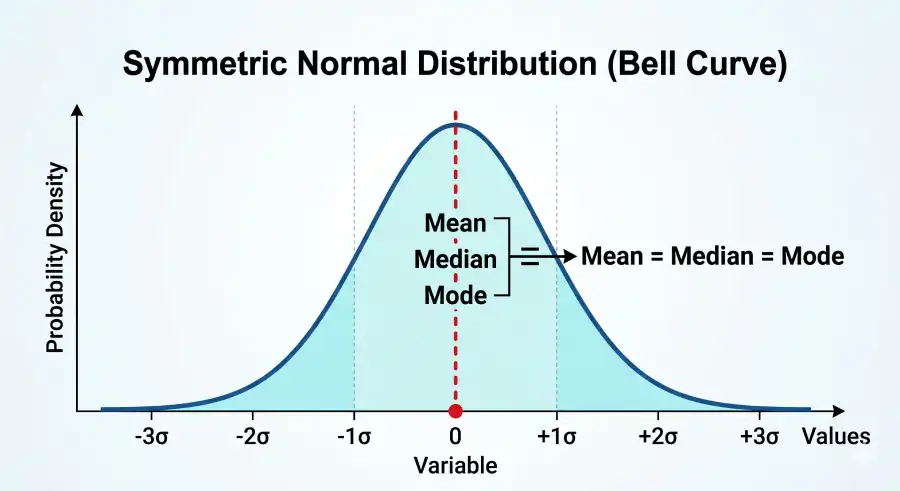
Symmetric Distributions: Mean = Median = Mode
In a perfectly symmetric, unimodal distribution (such as the normal distribution), the mean, median, and mode all coincide at exactly the same value — the center of the curve. This is because symmetry ensures no value is systematically pulled left or right, so the most common value, the middle value, and the arithmetic average all land at the same point. This is covered formally in any mathematical statistics text, including Wackerly, Mendenhall, and Scheaffer's Mathematical Statistics with Applications (8th ed., Cengage, 2008), which is standard reading at most university statistics programs.
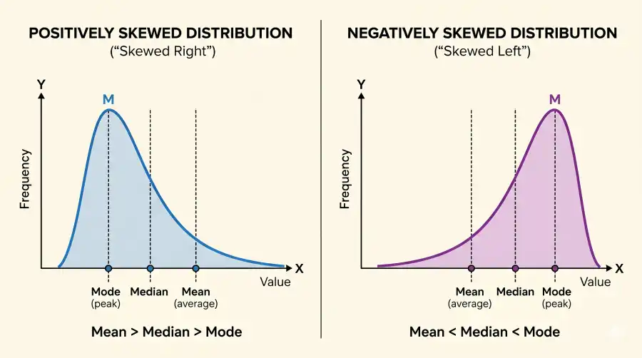
Skewed Distributions: How the Mode, Median, and Mean Separate
Skewness pulls the mean and, to a lesser degree, the median away from the mode. The mode always sits at the peak — where the data is densest. The mean gets dragged toward the tail because it responds to every value arithmetically. The median lands between them. This ordering gives rise to Pearson's empirical rule, covered in the next section.
Case Study — Income Data in the United States
Why median household income is reported instead of mean income
The U.S. Census Bureau reports median household income rather than mean household income in its official summary tables (U.S. Census Bureau, Income and Poverty). The reason is skewness: because a small number of households earn very high incomes, the mean is consistently higher than the median. The mode of the income distribution — the income level that appears most frequently — sits lower still, typically near the most common income bracket. Reporting the mean alone would give a figure that exceeds the actual income of the majority of households.
The Empirical Relationship: Mean, Median, and Mode
Karl Pearson derived an approximate relationship between the three measures of central tendency that holds for moderately skewed, unimodal distributions. This formula lets you estimate any one of the three values from the other two — useful when only summary statistics are available and the raw data is not.
Rearranges to: Median ≈ (Mode + 2·Mean) / 3 | Mean ≈ (3·Median − Mode) / 2
A dataset has a mean of 60 and a median of 65. Estimate the mode.
Apply the formula: Mode ≈ 3(Median) − 2(Mean) = 3(65) − 2(60) = 195 − 120 = 75
Check the direction: Mode (75) > Median (65) > Mean (60). This ordering is consistent with a negatively skewed distribution, where the left tail drags the mean down below the median and mode. The empirical relationship is internally consistent.
✓ Estimated Mode ≈ 75. Note that this is an approximation. For exact results, you need the raw data or the full frequency distribution.
Pearson's rule breaks down for bimodal or multimodal distributions (it assumes a single peak), for heavily skewed datasets, and for discrete distributions with very few distinct values. Do not apply it mechanically without first checking that the distribution is roughly unimodal and moderately skewed. If the raw data is available, compute the mode directly.
Ordering of Mean, Median, and Mode by Skewness
| Distribution Shape | Ordering | Example Context | Pearson Rule Applies? |
|---|---|---|---|
| Perfectly symmetric (normal) | Mean = Median = Mode | Heights in a large homogeneous population | Trivially — all three equal |
| Positively skewed (right tail) | Mode < Median < Mean | Income distributions, house prices | Yes, for moderate skew |
| Negatively skewed (left tail) | Mean < Median < Mode | Age at retirement; exam scores with a ceiling | Yes, for moderate skew |
| Bimodal | No fixed ordering | Heights of adults (male + female combined) | No — formula assumes unimodal |
| Uniform | Mean = Median; No mode | Outcomes of a fair die roll | Not applicable (no mode) |
When Should You Use the Mode Instead of the Mean?
The mean is the go-to measure of central tendency for most numerical data, but three specific situations make the mode the better — or the only — choice.
Categorical / Nominal Data
What is the most popular shirt color sold this month? The most common voting choice? These questions have no numeric order, so mean and median are undefined. The mode is the only valid answer.
Inventory & Demand Planning
A store stocking shoe sizes reorders based on the mode, not the mean. Knowing the average shoe size is 9.3 does not tell you what to put back on the shelf. The mode — the size that sold most often — does.
Discrete Data with Few Values
Survey responses on a 1–5 scale rarely have a meaningful mean (3.4 stars does not correspond to a real rating). The mode — the most common rating selected — is more directly interpretable.
Outlier-Contaminated Datasets
When one or two extreme values would distort the mean, the mode is stable. The mode of {2, 5, 5, 7, 10,000} is 5, regardless of the outlier. The mean is 2003.8, which misrepresents the bulk of the data.
Healthcare: Most Common Diagnosis
In a clinic's monthly patient log, the modal diagnosis tells staff which condition to prepare for most often — a planning input that neither mean nor median diagnosis codes would provide.
Voting and Elections
In a plurality election (first-past-the-post), the winner is the candidate chosen by the most voters — i.e., the modal choice. Mean and median are not defined for named candidates.
Mode Formula Glossary: All Notations Defined
The table below consolidates every term used in mode calculations so the formulas can be read without referring back to earlier sections. This format is designed for quick lookup when working through exam problems or grouped-data calculations.
| Symbol / Term | Notation | Meaning | Example Value |
|---|---|---|---|
| Mode (ungrouped) | Mo | The value that appears most often in raw data | Mo = 85 in {68, 72, 85, 85, 85, 90, 91} |
| Modal class | — | The class interval with the highest frequency in a grouped table | 4,000–5,000 (frequency = 22) |
| Lower class limit | l | The lowest value that can belong to the modal class | l = 4,000 |
| Modal class frequency | f₁ | The count of observations in the modal class | f₁ = 22 |
| Pre-modal frequency | f₀ | Frequency of the class immediately before the modal class | f₀ = 14 |
| Post-modal frequency | f₂ | Frequency of the class immediately after the modal class | f₂ = 10 |
| Class width | h | The range of each class interval (upper limit minus lower limit) | h = 1,000 |
| Empirical mode estimate | Mo ≈ 3Md − 2x̄ | Pearson's formula to approximate mode from median (Md) and mean (x̄) | 3(65) − 2(60) = 75 |
| Unimodal | |Mo| = 1 | Exactly one mode exists | {3, 5, 5, 5, 8} → Mo = 5 |
| Bimodal | |Mo| = 2 | Exactly two modes tied at the highest frequency | {10, 10, 25, 25} → Mo = 10, 25 |
| Multimodal | |Mo| ≥ 3 | Three or more modes | {2, 2, 4, 4, 6, 6} → Mo = 2, 4, 6 |
| No mode | Mo = ∅ | All values appear the same number of times (usually once) | {1, 2, 3, 4, 5, 6} |
Mode vs. Mean vs. Median: Full Comparison
The three measures of central tendency answer different questions about a dataset. None is universally superior — the right choice depends on the data type, the distribution's shape, and what the number will be used for. The table below captures the key distinctions that appear on exams and in applied statistics work.
| Property | Mode (Mo) | Median (Md) | Mean (x̄) |
|---|---|---|---|
| Definition | Most frequent value | Middle value when sorted | Sum ÷ count |
| Works on categorical data? | ✅ Yes | ❌ No (needs order) | ❌ No (needs numbers) |
| Affected by outliers? | No — completely immune | Slightly — resistant but not immune | Yes — highly sensitive |
| Unique value guaranteed? | No — can have 0, 1, or many | Yes — always one value | Yes — always one value |
| Best for | Categorical data; most common value; inventory | Skewed numerical data; ranked data; incomes | Symmetric numerical data; further calculations (e.g., SD) |
| Symmetric normal distribution | = Median = Mean | = Mode = Mean | = Mode = Median |
| Positively skewed distribution | Lowest of three | Middle value | Highest of three |
| Used in further statistics? | Rarely (no algebra) | Percentile calculations | SD, variance, t-tests, regression |
For a side-by-side comparison with worked examples across all three measures, see the Mean vs. Median vs. Mode guide on this site. If you need to compute all three simultaneously, the mean, median, and mode calculator accepts any dataset and returns all three values plus the range.
Frequently Asked Questions about the Mode
Yes — the mode is the only measure of central tendency that applies to nominal data. If a survey of 100 people about their favorite primary color returns 40 votes for red, 35 for blue, and 25 for yellow, the mode is red. There is no way to compute a "mean" or "median" primary color, but the mode is well-defined. This is covered in UCLA's OARC Statistical Methods guide, which lists the mode as the standard summary statistic for nominal measurement scales.
The mode is completely unaffected by outliers. Consider the dataset {3, 5, 5, 7}: mode = 5, mean = 5. Now add the outlier 10,000: {3, 5, 5, 7, 10,000}. The mode is still 5. The mean is now 2,004. This immunity is one reason the mode is preferred over the mean in datasets where extreme values occur but should not define the "typical" observation — for example, in quality control, where a single catastrophic failure should not define the typical product performance.
A uniform distribution has no mode. By definition, every value in a uniform distribution occurs with equal frequency. Since no value occurs more than any other, there is no single "most common" value. For example, in a perfectly fair coin flip (heads or tails, each 50%), neither outcome is the mode. Similarly, a dataset {4, 4, 7, 7, 9, 9} has three equally frequent values — it could be called trimodal, but some statisticians prefer to say it has no single dominant mode.
Bimodal means exactly two modes — two values share the highest frequency. Multimodal is the broader term covering any distribution with two or more modes (so bimodal is a specific type of multimodal). A dataset with three tied-highest frequencies is trimodal, which is multimodal but not bimodal. The distinction matters in practice: a bimodal income distribution suggests two distinct population sub-groups, while a trimodal or higher pattern may suggest a more complex underlying structure in the data.
Use the mode when: (1) your data is categorical and arithmetic is undefined, (2) you need to know what is most common rather than the average level, (3) your dataset has outliers that would distort the mean, or (4) your data is discrete with few possible values and a mean would not correspond to a real observation. Use the mean when the data is numerical, roughly symmetric, and you need a value for further calculations like standard deviation or hypothesis tests.
Sources and Further Reading
Academic and Institutional References
NIST/SEMATECH e-Handbook of Statistical Methods. "Measures of Location: Mode." National Institute of Standards and Technology. Available at: itl.nist.gov.
Penn State STAT 100: Statistical Concepts and Reasoning. Lesson 2.2: "Describing Data: Measures of Center." Available at: online.stat.psu.edu.
Sheffield, S. (2022). MIT 18.600: Probability and Random Variables, Lecture 3 Notes. Massachusetts Institute of Technology. Available at: math.mit.edu.
U.S. Census Bureau. Income and Poverty Statistics Documentation. Available at: census.gov.
UCLA Statistical Consulting Group (OARC). "What Statistical Analysis Should I Use?" — measurement scale guidance. Available at: stats.oarc.ucla.edu.
Wackerly, D., Mendenhall, W., & Scheaffer, R.L. (2008). Mathematical Statistics with Applications, 7th ed. Thomson Brooks/Cole. (Standard university text covering Pearson's empirical relationship, Chapter 1–2.)
Related Topics on Statistics Fundamentals
The mode is one piece of a broader toolkit in descriptive statistics. The guides below cover the concepts that appear most often alongside the mode in coursework and applied analysis.
Mean (Average)
Arithmetic, geometric, and weighted means with full formulas and step-by-step examples.
Median
The middle value for sorted data, resistant to outliers, and the standard for skewed distributions.
Standard Deviation
The primary measure of spread — how far individual values sit from the mean.
Variance
The squared average of deviations from the mean — the building block of standard deviation.
Types of Data
Nominal, ordinal, interval, and ratio scales — and which statistical operations apply to each.
Normal Distribution
The bell curve where mean = median = mode — and how the 68-95-99.7 rule applies.
Visit Statistics Fundamentals for the full library of guides, calculators, and statistical tables covering everything from outlier detection to hypothesis testing and regression analysis.