What Does a Static Threshold Assume About Your Data?
Every static threshold makes a hidden claim: that one value divides normal behavior from abnormal behavior at all times. In statistical terms, it assumes the metric has a single, stable distribution and that the threshold sits far enough into its tail.
That assumption rarely holds in practice. The distribution of a metric changes with the time of day, the day of the week, the release cycle and the workload. A reading of 85 percent CPU can be routine during a weekday business peak and a warning sign on a quiet Sunday night.
Most thresholds are also chosen by habit rather than measurement. Round numbers such as 80 or 90 percent come from vendor defaults or past incidents, not from the metric's own history. The result is a cut-off with no defined error rate, so you cannot say in advance how often it will fire without cause.
How Are IT Metrics Distributed?
IT metrics are rarely normal. Most of them have a hard lower bound, a long right tail and a shape that shifts over time. These features decide which statistical tools will work and which will mislead you.
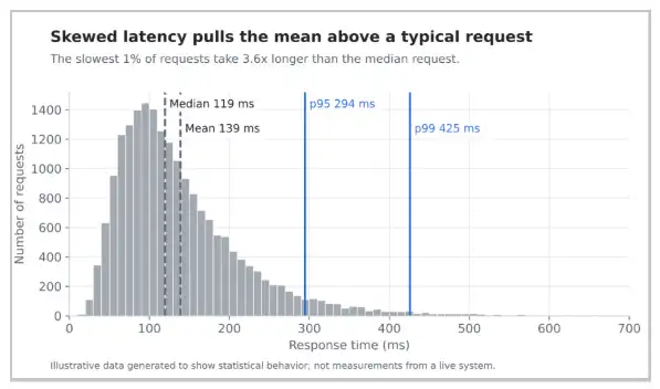
- Right skew. Response time, queue length and request latency cannot fall below zero but can spike far above the typical value. Most requests finish quickly, while a small share takes many times longer, a pattern known as positive skewness.
- Heavy tails. Extreme values appear more often than a normal distribution predicts, so rules based on the tail fire more than expected.
- Seasonality. Traffic, CPU and network throughput follow daily and weekly cycles tied to business hours and scheduled jobs.
- Bounded ranges. Utilization metrics sit between 0 and 100 percent, which compresses the distribution near its limits.
- Level shifts. A deployment, a configuration change or a new workload can move the normal operating level overnight.
Skew matters because it pulls the mean away from the center of the data. In a right-skewed latency distribution, the mean sits above the median, and neither one describes the slow requests that users notice. That is why monitoring teams track percentiles such as p95 and p99, the response times below which 95 and 99 percent of requests fall. This site's guide to percentiles explains how they are calculated.
Why Do Static Thresholds Miss Incidents and Raise False Alarms?
A static threshold fails in two directions at once, and both failures map directly to the Type I and Type II errors of hypothesis testing.
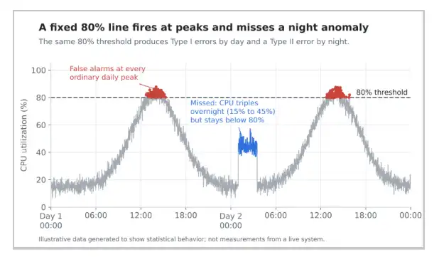
False positives (Type I errors). When the threshold sits inside the normal range of busy periods, it fires every time ordinary peak load arrives. Engineers learn that the alert means nothing, start muting it, and eventually miss the occurrence that matters. This is the root of alert fatigue.
False negatives (Type II errors). When the threshold sits high enough to stay quiet at peak, it cannot see problems during low-traffic hours. A process that triples its CPU use overnight, from 15 to 45 percent, is a clear anomaly. It never comes close to a 90 percent line.
How Do Mean and Standard Deviation Create a Baseline?
The simplest alternative to a fixed threshold is a baseline built from the metric's own history. You calculate the mean and the standard deviation of recent readings, then measure each new reading by how far it sits from that mean.
That distance is a z-score:
Here x is the new reading, μ is the baseline mean and σ is the baseline standard deviation. A z-score of 3 means the reading sits three standard deviations above normal, whatever the metric's units. That lets one rule work for CPU, memory, latency and error counts alike.
The common three-sigma rule flags any reading with an absolute z-score above 3. Its logic comes from the empirical rule: in a normal distribution, about 99.7 percent of values fall within three standard deviations of the mean. Only about 0.27 percent fall outside by chance.
That figure depends on normality, which IT metrics rarely have. Chebyshev's inequality gives a guarantee that holds for any distribution: at least 1 − 1/k² of values lie within k standard deviations of the mean. For k = 3, that is only 88.9 percent, which leaves up to 11.1 percent outside. A three-sigma rule on skewed data can therefore fire far more often than the textbook figure suggests.
What Should You Use When the Data Is Skewed?
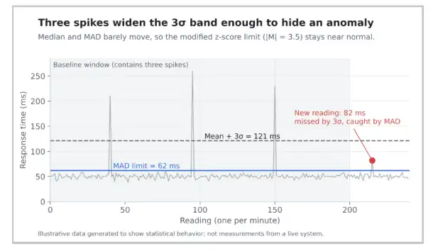
The mean and standard deviation are sensitive to the very spikes you are trying to detect. One large spike in the baseline window raises the mean and inflates the standard deviation. The band widens, and the next anomaly slips through inside it. Statisticians call this effect masking.
Robust statistics avoid the problem by replacing the mean with the median and the standard deviation with the median absolute deviation (MAD). The MAD is the median of each reading's absolute distance from the median. Because both measures depend on the middle of the data, a handful of extreme values barely move them.
The modified z-score uses the median and MAD in place of the mean and standard deviation:
Here x̃ is the median of the baseline window. The constant 0.6745 puts the score on the same scale as an ordinary z-score when the data is normal. Iglewicz and Hoaglin proposed treating values with an absolute M above 3.5 as potential outliers, and that cut-off is a widely used starting point.
Percentile bands are a second option. Instead of measuring distance from the center, you alert when a reading exceeds a high percentile of the same metric's history, such as the 99th. Percentiles make no assumption about the shape of the distribution, which suits skewed latency data well.
How Do You Account for Time of Day and Day of Week?
A baseline built from one undivided window still compares Monday morning with Sunday night. The fix is to compare each reading with readings taken at the same point in the cycle.
Seasonal baselines. You group history by hour of the day, or by hour of the week, and compute a separate median and spread for each slot. A reading at 10 a.m. on a Tuesday is then judged against previous Tuesdays at 10 a.m. This captures the business-hours pattern that a single baseline cannot.
Rolling windows. You recompute the baseline over a sliding window, such as the last four weeks, so it follows gradual growth and drops old behavior. The window length is a trade-off. Short windows adapt quickly but can absorb slow-building problems into the baseline. Long windows stay stable but take longer to accept a legitimate level shift after a release.
Exponentially weighted moving averages. An EWMA gives recent readings more weight than older ones through a smoothing factor between 0 and 1. It tracks a drifting level without storing a long history, and its residuals can feed the same z-score rules described above.
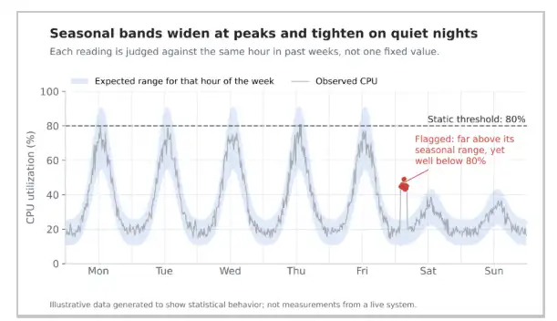
A seasonal band widens where the metric is naturally variable and narrows where it is steady. That is the behavior a fixed line cannot provide: tolerance at peak hours and sensitivity during quiet ones.
Why Does a Good Baseline Still Produce False Alarms?
Even a well-built baseline fires by chance, and the volume adds up quickly. A metric sampled once a minute produces 1,440 readings a day. At the 0.27 percent false positive rate of a three-sigma rule on normal, independent data, that is about 3.9 chance breaches per metric per day. Across 1,000 metrics, it is roughly 3,900.
This is the multiple comparisons problem. Each test has a small error rate, but running thousands of them produces a steady stream of false positives.
The base rate makes it worse. True incidents are rare compared with the number of readings checked. When the condition you are looking for is rare, even an accurate test produces more false alarms than true detections. Medical screening faces the same issue, and the false positive paradox calculator on this site shows how sharply the share of true alerts falls as the base rate drops.
Monitoring teams counter this in three ways:
- Persistence rules. An alert fires only when several recent readings breach the band, such as three of the last five, which filters out single-sample spikes.
- Correlation across signals. An anomaly in latency that coincides with anomalies in CPU, error rate and queue depth is far more likely to point to a genuine problem than any one of them alone.
- Severity by distance. A reading at a z-score of 3.2 and one at 9 should not page the same person with the same urgency.
Where Does Machine Learning Take Over?
Statistical baselines work well for one metric at a time. Their limits appear when behavior depends on several signals together, when seasonality is irregular, or when thousands of metrics each need a baseline that someone has to maintain.
Machine learning methods extend the same ideas rather than replacing them. Models learn expected ranges from history, account for several seasonal cycles at once and score multivariate patterns that no single-metric rule can see, such as rising latency while traffic stays flat. They can also group related anomalies so that one underlying fault produces one alert instead of dozens.
Most observability platforms now offer both approaches side by side. In Motadata's unified observability platform, for example, teams can set fixed-threshold policies for hard limits and AI/ML policies for anomaly detection, dynamic baselines and alert correlation. Fixed thresholds still have a place. A disk at 100 percent capacity or an expired certificate needs no statistical model to qualify as a problem.
How Do You Set Better Alert Thresholds?
Use these checks when you review an existing alert or design a new one:
- Plot the metric's history as a histogram before choosing a threshold, and note its skew, range and outliers.
- Keep fixed thresholds for hard limits, such as full disks, expired certificates and breached SLA ceilings.
- Use the median and MAD, or percentiles, instead of the mean and standard deviation for skewed metrics.
- Build baselines by hour of day or hour of week for any metric with a business-hours pattern.
- Choose a rolling window that follows growth without absorbing slow-building problems.
- Require persistence across several readings before an alert fires.
- Estimate how often the rule will fire by chance, then multiply by the number of metrics it covers.
- Review alert outcomes regularly and track how many alerts led to action.
A static threshold is a statistical guess with an unknown error rate. A baseline that reflects the metric's own distribution, cycles and tails turns that guess into a measured decision. The statistics involved are the ones taught in any introductory course, applied to data that changes every minute.
- Static threshold — a fixed value that divides normal from abnormal at all times; fails because distributions shift across the day
- Type I error (false positive) — alert fires on normal peak load; root cause of alert fatigue
- Type II error (false negative) — alert misses slow overnight anomalies that never reach the fixed line
- Z-score — distance of a reading from the baseline mean, measured in standard deviations
- Modified z-score — replaces mean and SD with median and MAD; resistant to spikes in the baseline window
- Seasonal baseline — separate median and spread per hour-of-week slot; captures business-hours patterns
- Multiple comparisons problem — 1,000 metrics at 0.27% false positive rate produces ~3,900 chance alerts per day
- Base rate — true incidents are rare, so even accurate rules produce more false alarms than true detections
Static vs. Dynamic Thresholds: At a Glance
| Property | Static Threshold | Dynamic Baseline |
|---|---|---|
| Setup effort | Low — one number | Higher — requires history |
| Adapts to time of day | No | Yes, with seasonal grouping |
| Handles skewed data | No | Yes, with median / MAD |
| Detects overnight anomalies | Only if value exceeds fixed line | Yes — relative to quiet-period baseline |
| Known false positive rate | No | Approximately, via z-score |
| Best suited for | Hard limits (disk full, cert expired) | Behavioral metrics (latency, CPU, errors) |