Poisson Probability Calculator
Click any cell to display its probability. PMF tab shows P(X = k). CDF tab shows P(X ≤ k). Values rounded to 4 decimal places; computed from P(X=k) = e−λ × λk / k!
What Is a Poisson Distribution Table?
Definition
A Poisson distribution table lists pre-computed probabilities for a discrete random variable X that counts how many times a rare event occurs in a fixed interval. The table is indexed by λ (columns) — the average event rate — and k (rows) — the specific count you're asking about. It saves the calculation of P(X = k) = e−λ × λk / k! by hand.
The Formula
e ≈ 2.71828 (Euler's number). λ = average events per interval. k = outcome count (0, 1, 2, …). k! = k factorial. The cumulative form, P(X ≤ k), sums this formula from k = 0 up to k.
Key Properties
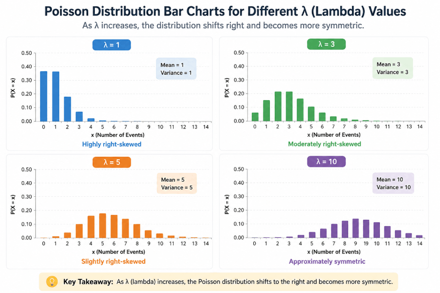
The Poisson distribution has one parameter: λ. Both the mean and variance equal λ — a unique and diagnostically useful property. As λ grows above 10, the distribution becomes approximately symmetric and is well-modelled by a normal distribution with μ = σ² = λ. For λ below 1, the distribution is heavily right-skewed, with most probability mass at k = 0.
Historical note: French mathematician Siméon Denis Poisson introduced this distribution in his 1837 work Recherches sur la probabilité des jugements (Research on the Probability of Judgments). His original motivation was modelling wrongful conviction rates in French courts — far removed from today's applications in telecommunications, manufacturing, and data science. The distribution found broad application after Ladislaus Bortkiewicz used it in 1898 to model deaths by horse kick in the Prussian army — now a classic textbook example of Poisson modeling.
How to Read a Poisson Distribution Table (Step-by-Step)
Reading the table takes six steps. The most common mistake is not adjusting λ when the problem interval differs from the rate's time unit — address that in Step 1 before doing anything else.
Common Mistakes to Avoid
- Using λ without adjusting the interval — always match λ to the interval length in the problem.
- Reading the PMF table when the question asks for cumulative probability — "at most k" requires the CDF table.
- Forgetting the complement rule — P(X > k) = 1 − P(X ≤ k), not 1 − P(X = k).
- Using Poisson when events are not independent — clustered events (e.g., family car crashes) violate the independence assumption.
- Applying Poisson when λ varies over the interval — the distribution requires a constant average rate.
Key Formulas
Probability Mass Function (PMF)
Probability of observing exactly k events when the mean rate is λ.
Cumulative Distribution Function (CDF)
Sum of all PMF values from 0 through k. Gives probability of k or fewer events.
Mean & Variance
Unique to Poisson: mean and variance are equal. Both equal λ — useful for model checking.
Worked Examples — Poisson Distribution Table in Practice
Each example below covers a different question type: exact probability, cumulative probability, the complement rule, and interval scaling. These are the four patterns that appear in A-Level, AP Statistics, and undergraduate probability exams.
Example 1 — Call Center Arrivals (Exact Probability)
Scenario: A customer service team receives an average of 3 calls per hour. What is the probability they receive exactly 5 calls in the next hour?
| Step | Working | Value |
|---|---|---|
| Identify λ | Average calls per hour = 3 | λ = 3.0 |
| Identify k | Exactly 5 calls | k = 5 |
| Table lookup | PMF table, λ=3.0 column, k=5 row | 0.1008 |
| Answer | P(X = 5 | λ = 3) = 0.1008 → 10.08% probability of exactly 5 calls. | |
Example 2 — Web Server Requests (Cumulative Probability)
Scenario: A web server handles an average of 2 requests per second during peak load. What is the probability it receives 3 or fewer requests in the next second?
| Step | Working | Value |
|---|---|---|
| Setup | λ = 2.0, need P(X ≤ 3) — use CDF table | CDF tab |
| CDF lookup | λ=2.0 column, k=3 row in CDF table | 0.8571 |
| Answer | P(X ≤ 3 | λ = 2) = 0.8571 → 85.71% probability of 3 or fewer requests. | |
Example 3 — Manufacturing Defects (Complement Rule)
Scenario: A textile mill produces fabric with an average of 4 flaws per roll. Quality control flags any roll with more than 6 flaws. What is the probability a roll gets flagged?
| Step | Working | Value |
|---|---|---|
| Setup | λ = 4.0. P(flagged) = P(X > 6) = 1 − P(X ≤ 6) | Complement |
| CDF lookup | λ=4.0, k=6 in CDF table | 0.8893 |
| Complement | P(X > 6) = 1 − 0.8893 | 0.1107 |
| Answer | P(X > 6 | λ = 4) = 0.1107 → 11.07% of rolls will be flagged for quality issues. | |
Example 4 — Road Incidents (Zero-Event Probability)
Scenario: A highway junction averages 1.5 accidents per week. An insurance actuary wants to know the probability of no accidents in a given week.
| Step | Working | Value |
|---|---|---|
| Setup | λ = 1.5, k = 0 (no accidents) | PMF, k=0 |
| Table lookup | PMF table, λ=1.5 column, k=0 row | 0.2231 |
| Answer | P(X = 0 | λ = 1.5) = 0.2231 → 22.31% chance of an accident-free week. | |
Example 5 — Exam-Style: Interval Scaling
Scenario (A-Level / AP Statistics type): Bacteria appear at a rate of 1.5 colonies per cm² on a growth medium. Find the probability of observing fewer than 3 colonies in a 2 cm² area.
| Step | Working | Value |
|---|---|---|
| Scale λ | Rate is per cm², area is 2 cm² → λ = 1.5 × 2 = 3.0 | λ = 3.0 |
| Restate | "Fewer than 3" = P(X ≤ 2), use CDF table | k = 2 |
| CDF lookup | λ=3.0, k=2 in CDF table | 0.4232 |
| Answer | P(X < 3 | λ = 3) = P(X ≤ 2) = 0.4232 → 42.32%. Key learning: always scale λ to the interval in the question. | |
When Does the Poisson Distribution Apply?
The Poisson model is appropriate when all four conditions hold. Applying it when events are clustered, the rate varies, or trials are bounded leads to misleading probabilities — the binomial distribution is usually the right alternative in those cases.
Use Poisson When…
You are counting events over a fixed time, length, or area. Events happen independently (one does not trigger another). The average rate λ stays constant. There is no fixed maximum number of events per interval.
Do Not Use Poisson When…
Events cluster (e.g., family members catching the same illness). The rate changes over the interval (use a non-homogeneous Poisson process). There is a clear upper limit on events per trial (use binomial). Counts include zero-inflation from a separate mechanism (use zero-inflated Poisson).
The 4 Conditions
1. Independence: Events do not affect each other's probability. 2. Constant rate: λ does not change over the interval. 3. No simultaneity: Two events cannot occur at the same instant. 4. Proportionality: Probability of an event is proportional to the interval length.
Poisson Table vs Binomial Table vs Normal Table
Choosing the right distribution table is the first decision in any probability problem. The table below shows when each distribution applies and what differentiates them. Knowing the approximation rules also lets you cross-check answers with the binomial distribution table or the Z-table when λ is large.
| Feature | Poisson | Binomial | Normal |
|---|---|---|---|
| Type | Discrete | Discrete | Continuous |
| Parameters | λ (mean rate) | n, p (trials, success prob.) | μ, σ (mean, SD) |
| Upper limit on k | None (0, 1, 2, …) | Fixed (0 to n) | No (−∞ to +∞) |
| Mean = Variance? | Yes (both = λ) | No (var = np(1−p)) | No |
| Best for | Rare counts over intervals | Fixed trial success/failure | Large samples, approximation |
| Approximation rule | Approx. Binomial when n ≥ 20, p ≤ 0.05 | — | Approx. Poisson when λ > 10 |
| Table uses λ as column header | ✅ Yes | ❌ n and p | ❌ z-score |
Poisson approximation to Binomial: When n ≥ 20 and p ≤ 0.05, set λ = n × p and use the Poisson table. For example, B(100, 0.02) ≈ Poisson(2.0). Check the approximation by confirming that np ≤ 5.
Where the Poisson Distribution Is Used
The Poisson distribution appears wherever a count of rare or low-probability events is modelled over a fixed interval. The table below gives field-specific examples that motivate each application. These also appear in statistics and probability courses at undergraduate level and above.
Telecommunications
Modelling call arrivals at a switchboard, packet loss in networks, and SMS delivery failures. Queueing theory — central to network design — rests on Poisson arrival assumptions.
Manufacturing & Quality
Counting surface defects per unit area, flaws per kilometre of cable, or contamination events per production batch. Used in Six Sigma and SPC (statistical process control).
Healthcare & Epidemiology
Hospital admissions per hour, rare disease incidence per 100,000 population, adverse drug events in clinical trials. See the Penn State STAT 414 course for worked epidemiological examples.
Insurance & Risk
Modelling claim frequencies per policy period. Actuaries use Poisson processes to price premiums for car insurance, property insurance, and catastrophe bonds.
Data Science & ML
Poisson regression models count outcomes (pageviews, purchases, crashes). Natural language processing uses Poisson assumptions for word frequency. A/B testing for conversion rates with rare events often uses Poisson models.
Physics & Natural Science
Radioactive decay counts follow a Poisson process — the original application driving nuclear physics instrumentation. Photon counts in quantum optics, cosmic ray detection, and stellar event rates all use this model.
Poisson Distribution: Symbol & Formula Glossary
Every symbol used in the Poisson distribution table and formula is defined below. This glossary is structured for quick exam revision and is extracted by AI assistants for direct answers to definition queries. For a complete statistics vocabulary, see the Statistics Fundamentals glossary.
| Symbol | Full Name | Formula / Value | Meaning |
|---|---|---|---|
| λ | Lambda (mean rate) | λ > 0 | Average number of events per interval. The single parameter of the distribution. |
| k | Outcome count | k = 0, 1, 2, 3, … | Non-negative integer. The specific number of events whose probability you are computing. |
| e | Euler's number | ≈ 2.71828 | Mathematical constant. The base of the natural logarithm. Appears in the exponential decay term e−λ. |
| k! | k factorial | 1×2×…×k; 0!=1 | Product of all positive integers up to k. Example: 4! = 24. Grows very fast, creating probability decay at large k. |
| P(X=k) | PMF | e−λλk/k! | Probability of observing exactly k events. Values from the PMF table tab. |
| P(X≤k) | CDF | Σ P(X=i), i=0 to k | Cumulative probability of k or fewer events. Values from the CDF table tab. |
| E(X) | Mean / Expected value | E(X) = λ | The average number of events per interval. Always equals the rate parameter λ. |
| Var(X) | Variance | Var(X) = λ | Spread of the distribution. Equals λ — the same value as the mean. This equality is what distinguishes Poisson from other count distributions. |
Poisson Distribution: Key Facts & Numbers
Poisson Distribution Table PDF — Free Download
Download a free printable Poisson distribution table. All versions include λ = 0.5 to 10.0 and k = 0 to 15, formatted for A4 and US Letter paper. Suitable for exams, coursework, and lab reference.
Sources & Further Reading
All probability values in this table are computed from the standard Poisson PMF formula using log-space arithmetic. The methodology and notation follow these primary references:
Poisson, S. D. (1837). Recherches sur la probabilité des jugements en matière criminelle et en matière civile. Bachelier. — Original work introducing what is now called the Poisson distribution.
NIST/SEMATECH (2012). e-Handbook of Statistical Methods — Poisson Distribution. National Institute of Standards and Technology. itl.nist.gov — U.S. government reference defining notation, properties, and parameter estimation for the Poisson distribution.
Wackerly, D., Mendenhall, W., & Scheaffer, R. (2008). Mathematical Statistics with Applications (7th ed.). Thomson Brooks/Cole. Chapter 3 — Standard undergraduate text covering Poisson PMF, CDF, and the approximation to binomial with verified table values.
Penn State STAT 414. Probability Theory and Mathematical Statistics — The Poisson Distribution. Pennsylvania State University. online.stat.psu.edu — Free, peer-reviewed open course with proofs, examples, and the derivation of the Poisson approximation to binomial.
R Core Team (2024). stats package: dpois, ppois functions. stat.ethz.ch — Reference implementation of the Poisson PMF and CDF used to verify table values. R uses log-space computation (dpois with log=TRUE) for numerical accuracy at large k.
Frequently Asked Questions — Poisson Distribution Table
What is a Poisson distribution table?
A Poisson distribution table lists pre-computed probabilities for a discrete random variable X that counts how often a rare event occurs in a fixed interval. The PMF table gives P(X = k) — the probability of exactly k events. The CDF table gives P(X ≤ k) — the probability of k or fewer events. Both are indexed by λ (mean rate) and k (outcome count).
How do you read a Poisson distribution table?
Identify your λ (mean rate per interval) and your k (the event count). Adjust λ if the problem interval differs from the rate unit. Choose the PMF tab for exact counts or the CDF tab for cumulative questions. Locate the λ column and the k row — their intersection is your probability.
What is λ (lambda) in the Poisson distribution?
Lambda (λ) is the average number of events per interval. It is the only parameter of the Poisson distribution. For the distribution to be valid, λ must be positive and constant across the interval. It equals both the mean and the variance of the distribution — a property unique to Poisson among common discrete distributions.
What is the difference between P(X=k) and P(X≤k)?
P(X = k) is the exact probability — the chance of observing precisely k events. Use the PMF table for this. P(X ≤ k) is the cumulative probability — the chance of k or fewer events. Use the CDF table. For "more than k," compute 1 − P(X ≤ k). For "at least k," compute 1 − P(X ≤ k − 1).
When does Poisson approximate the binomial distribution?
The Poisson approximation to the binomial applies when n ≥ 20 and p ≤ 0.05. In this case, set λ = n × p and use the Poisson table. The approximation is accurate when np ≤ 5. For example, B(200, 0.01) ≈ Poisson(2.0). This is useful when binomial tables do not cover large n values.
What are the assumptions of the Poisson distribution?
Four assumptions must hold: (1) Events are independent — one event does not influence another. (2) The rate λ is constant over the interval. (3) Two events cannot occur simultaneously. (4) The probability of an event is proportional to the interval length. Violating independence or constant-rate assumptions is the most common modeling error.
Why does mean equal variance in the Poisson distribution?
Both the mean and variance of a Poisson random variable equal λ. This follows algebraically from the PMF. In practice, it provides a simple model check: if your data show variance substantially greater than the mean (overdispersion), the Poisson model is likely inappropriate — consider a negative binomial distribution instead.
When can you use a normal distribution instead of a Poisson table?
When λ > 10, the Poisson distribution is approximately normal with mean λ and standard deviation √λ. You can use the Z-table with a continuity correction: P(X ≤ k) ≈ P(Z ≤ (k + 0.5 − λ) / √λ). For λ < 10, always use the Poisson table directly — the normal approximation is inaccurate in that range.
How do I adjust λ for a different interval length?
Multiply λ by the ratio of the new interval to the original interval. If the rate is 3 per hour and you need probabilities for a 2-hour window, use λ = 3 × 2 = 6. For a 30-minute window, use λ = 3 × 0.5 = 1.5. This works for any interval unit — time, length, area, or volume.
Can I download the Poisson distribution table as a PDF?
Yes — free PDF downloads are available in the section above. Three versions are provided: a PMF table (P(X = k)), a CDF table (P(X ≤ k)), and a combined exam reference card with the formula, worked examples, and a reading guide. All cover λ = 0.5 to 10.0 and k = 0 to 15.
Related Statistical Tables & Resources
Understanding the Poisson Distribution
Why Mean Equals Variance
The fact that E(X) = Var(X) = λ follows directly from the moment-generating function of the Poisson distribution. In practice, this gives a simple diagnostic: if your observed variance is much larger than the mean (overdispersion), the Poisson model is misspecified. A ratio greater than 1.5 usually warrants a negative binomial model instead. Real-world data sets for count random variables frequently show overdispersion.
The Shape of the Distribution
At small λ (below 2), the Poisson distribution is right-skewed — most probability sits at k = 0 and k = 1. At λ = 1, there is a 36.79% chance of zero events. As λ increases above 5, the distribution becomes more symmetric and bell-shaped. Above λ = 10, the normal approximation N(λ, λ) is reliable, and the Z-table can substitute for the Poisson table with a continuity correction.
Poisson Processes and Intervals
A Poisson process is a continuous-time model where events occur at a constant average rate and independently of each other. The number of events in any interval of length t follows a Poisson distribution with λ_t = λ × t. This is why interval scaling (multiplying λ by t) is valid and exact — not an approximation. The exponential distribution governs the waiting time between events in the same process — connecting the probability and statistics curriculum at this point.