What Is Expected Value? (Definition)
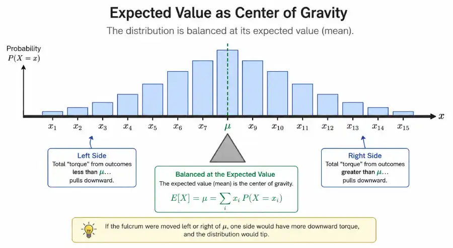
The plain-English translation: multiply each possible outcome by the probability that outcome occurs, then add all those products together. The result is a single number — the "center of gravity" of the entire probability distribution.
Consider a fair six-sided die. The outcomes are 1 through 6, each with probability 1/6. Multiplying and summing: E(X) = 1(1/6) + 2(1/6) + 3(1/6) + 4(1/6) + 5(1/6) + 6(1/6) = 21/6 = 3.5. Roll that die 10,000 times and record every result; the average of all 10,000 numbers will be extremely close to 3.5.
- Notation: E(X), E[X], μ (mu), or <X> — all mean the same thing
- Formula (discrete): E(X) = Σ x·P(x) — sum of (outcome × probability)
- Formula (continuous): E(X) = ∫ x · f(x) dx — integral replaces summation
- Probabilities must sum to 1: Σ P(x) = 1 — this is non-negotiable
- Positive EV: The activity gains value on average over repeated trials
- Negative EV: The activity loses value on average — stay away or price it accordingly
- EV = 0: A "fair game" — neither side has a systematic advantage
The Expected Value Formula Explained
Discrete Random Variables: E(X) = Σ x·P(x)
E(X) = expected value (also written μ)Σ = "sum of" — add every termx = a specific outcome valueP(x) = probability that outcome x occursThe summation symbol Σ (sigma) tells you to repeat the multiplication for every possible value of x and then add the results. If a random variable can take five different values, you get five terms that you add together. If it can take 100 values, you get 100 terms. The formula scales to any number of outcomes.
Continuous Random Variables: E(X) = ∫ x · f(x) dx
∫ = integral (continuous analogue of Σ)f(x) = probability density function at xdx = infinitesimally small x intervalMost introductory statistics courses and real-world applications focus on the discrete case. The continuous version requires calculus but follows the same conceptual logic: weight each possible value by how likely it is, then accumulate those weighted values across the entire distribution.
Before computing any expected value, verify that Σ P(x) = 1.0. If your probabilities add to 0.9 or 1.1, the distribution is invalid and your EV calculation will be wrong. This is the single most common error on statistics exams and in real business models.
Expected Value Across Different Contexts
The same E(X) = Σ x·P(x) structure appears in every field — only the labels change. The table below maps how expected value notation and interpretation shift across four major application domains.
| Context | Discrete Formula | What x Represents | What P(x) Represents |
|---|---|---|---|
| Statistics / Probability Theory | E(X) = Σ x·P(x) | Numeric outcome of a random variable | Probability mass at that outcome |
| Finance / Investment Analysis | EV = Σ Rᵢ·Pᵢ | Return or payoff in dollars | Probability that scenario i occurs |
| Games of Chance / Gambling | EV = Σ (Net win)·P | Net gain/loss per play (in dollars) | Probability of that game outcome |
| Insurance / Actuarial Science | E(Loss) = Σ Lᵢ·Pᵢ | Claim amount (in dollars) | Probability that claim occurs |
The mathematical framework of expected value was formalized by Blaise Pascal and Pierre de Fermat in their 1654 correspondence on the "Problem of Points." The modern axiomatic treatment traces to Andrey Kolmogorov's 1933 foundational work on probability theory. See also: MIT OpenCourseWare — Statistics for Applications and OpenStax Introductory Statistics, Chapter 4.
How to Calculate Expected Value: 4 Steps
Every expected value calculation follows the same four-step process. Work through these steps in order and you will never miss a term or make an arithmetic error.
List All Outcomes
Write down every value the random variable X can take. Do not skip or combine outcomes — each unique payoff gets its own row.
Assign Probabilities
Record the probability for each outcome. Check that Σ P(x) = 1 before proceeding. This is non-negotiable.
Multiply Each Row
For each outcome, compute the product x × P(x). This gives you the weighted contribution of that outcome to the total average.
Sum All Products
Add every x·P(x) value from Step 3. The total is the expected value. Label it E(X) or μ.
Worked Examples
Example 1 — The Classic: Expected Value of a Die Roll
What is the expected value of one roll of a fair six-sided die?
| Outcome (x) | Probability P(x) | Product x · P(x) |
|---|---|---|
| 1 | 1/6 ≈ 0.1667 | 1 × 0.1667 = 0.1667 |
| 2 | 1/6 ≈ 0.1667 | 2 × 0.1667 = 0.3333 |
| 3 | 1/6 ≈ 0.1667 | 3 × 0.1667 = 0.5000 |
| 4 | 1/6 ≈ 0.1667 | 4 × 0.1667 = 0.6667 |
| 5 | 1/6 ≈ 0.1667 | 5 × 0.1667 = 0.8333 |
| 6 | 1/6 ≈ 0.1667 | 6 × 0.1667 = 1.0000 |
| TOTAL | 6/6 = 1.0000 | E(X) = 3.5000 |
Outcomes: x can be 1, 2, 3, 4, 5, or 6 — the six faces of a standard die.
Probabilities: Each face is equally likely, so P(x) = 1/6 for every outcome. Sum = 6 × (1/6) = 1. ✓
Products: Compute x·P(x) for each row (see table above).
Sum: 0.1667 + 0.3333 + 0.5000 + 0.6667 + 0.8333 + 1.0000 = 3.5
✓ E(X) = 3.5. This is a theoretical average — you can never roll a 3.5 on a single turn. But if you roll 10,000 times, the average of all your results will converge to 3.5.
Example 2 — Coin Flip: Expected Heads in Three Tosses
You flip a fair coin three times. What is the expected number of heads?
Let X = number of heads. X follows a binomial distribution with n = 3, p = 0.5.
| Heads (x) | Ways (combinations) | Probability P(x) | x · P(x) |
|---|---|---|---|
| 0 | TTT → 1 way | 1/8 = 0.125 | 0 × 0.125 = 0.000 |
| 1 | HTT, THT, TTH → 3 ways | 3/8 = 0.375 | 1 × 0.375 = 0.375 |
| 2 | HHT, HTH, THH → 3 ways | 3/8 = 0.375 | 2 × 0.375 = 0.750 |
| 3 | HHH → 1 way | 1/8 = 0.125 | 3 × 0.125 = 0.375 |
| TOTAL | 8 outcomes | 1.000 | E(X) = 1.500 |
✓ E(X) = 1.5 heads per 3-flip session. Confirms the binomial shortcut: E(X) = n·p = 3 × 0.5 = 1.5.
Example 3 — Gambling: American Roulette
You bet $1 on a single number in American roulette. What is your expected value?
An American roulette wheel has 38 pockets: numbers 1–36, plus 0 and 00. A winning single-number bet pays 35 to 1 (you receive $35 profit plus your $1 stake back). A loss means your $1 is gone.
| Outcome | Net Gain/Loss (x) | Probability P(x) | x · P(x) |
|---|---|---|---|
| Win (your number hits) | +$35 | 1/38 ≈ 0.02632 | +$35 × 0.02632 = +$0.9211 |
| Lose (any other number) | −$1 | 37/38 ≈ 0.97368 | −$1 × 0.97368 = −$0.9737 |
| TOTAL | 1.0000 | E(X) = −$0.0526 |
✓ E(X) = −$0.0526 per $1 wagered. This is the house edge: for every dollar bet on American roulette, the player loses 5.26 cents on average over time. The casino's expected value is exactly +$0.0526 per $1 wagered — guaranteed profit through volume.
The negative EV of −5.26% does not mean you will lose exactly 5.26 cents on your next spin. It means that over 1,000 or 10,000 spins, the casino's net profit will converge to 5.26% of total dollars wagered. A single player might win or lose any amount in one session — the Law of Large Numbers ensures the casino's revenue is predictable across millions of bets.
Example 4 — Business: Product Launch Decision
Should an entrepreneur launch a new product? Three market scenarios are possible.
| Scenario | Payoff (x) | Probability P(x) | x · P(x) |
|---|---|---|---|
| Strong demand (breakout success) | +$200,000 | 0.25 | +$50,000 |
| Moderate demand (break-even) | +$20,000 | 0.45 | +$9,000 |
| Weak demand (product flops) | −$80,000 | 0.30 | −$24,000 |
| TOTAL | 1.00 | E(X) = +$35,000 |
Interpretation: The launch has a positive expected value of +$35,000. Across many similar decisions made with this probability structure, the entrepreneur expects to gain $35,000 per launch on average. Whether to proceed still depends on risk tolerance and whether a single bad outcome is survivable — but the EV is favorable.
✓ E(X) = +$35,000. Positive EV — the launch is mathematically favorable when assessed over repeated similar decisions.
Interactive Expected Value Calculator
Enter your outcomes and probabilities below. The calculator computes Σ x·P(x) in real time. You can add up to 10 rows. Make sure probabilities sum to exactly 1.0 before calculating.
Expected Value Calculator — Discrete Random Variable
Rules of Expectation
Three algebraic properties of expected value are used constantly in more advanced probability and statistics work. Knowing these eliminates the need to rebuild the entire distribution table for transformed or combined variables.
Linearity of Expectation
The expected value of a sum always equals the sum of expected values — even when X and Y are not independent. This is one of the most powerful and universally applicable properties in probability theory.
Linear Transformation
Scaling a variable by constant a scales its expected value by a. Shifting by constant b shifts the expected value by b. Example: If E(X) = 3 and Y = 2X + 5, then E(Y) = 2(3) + 5 = 11.
Constant Expected Value
If c is a constant (not random), its expected value is simply c itself. A constant has no uncertainty — it always takes that exact value, so the weighted average is the value itself.
Product of Independent Variables
When X and Y are independent, the expected value of their product equals the product of their expected values. This does NOT hold in general when variables are dependent.
Because E(X + Y) = E(X) + E(Y) holds for any two random variables regardless of dependence, you can always decompose a complex problem. Expected number of heads in 100 coin flips? E(X) = 100 × E(one flip) = 100 × 0.5 = 50. No need to build a 101-row distribution table.
Positive vs Negative Expected Value
What Does a Negative Expected Value Mean?
| E(X) Sign | Meaning | Real-World Example |
|---|---|---|
| E(X) > 0 (Positive) | Average gain over many trials; activity has long-run upside | Positive-EV poker play, index fund investing, insurance underwriting |
| E(X) < 0 (Negative) | Average loss over many trials; activity has long-run downside | Casino slots (player side), lottery tickets, payday loans (borrower side) |
| E(X) = 0 (Fair Game) | No systematic advantage for either party over repeated play | Theoretical fair coin-flip bet at even odds; zero-sum trading with no fees |
A player with negative EV can absolutely win on a single session or even many consecutive sessions. Negative EV is a statement about the long-run average, not any individual outcome. This is exactly why gamblers are drawn in — short-run variance masks the structural disadvantage.
Expected Value and the Law of Large Numbers
Why a Single Trial Never Equals E(X)
You cannot roll the expected value of 3.5 on a single die throw. You cannot flip 1.5 heads in a single three-flip session. The expected value is not a prediction for any individual event — it is the mathematical limit of what the sample mean approaches as the number of trials grows without bound.
As n → ∞, the sample mean x̄ converges to E(X) in probability.
Formally: for any small ε > 0, P(|x̄ₙ − μ| > ε) → 0 as n → ∞. In plain English: the more trials you run, the closer your observed average gets to the theoretical expected value, and eventually the gap becomes arbitrarily small with probability 1. This result, rigorously established by Jakob Bernoulli (1713) and formalized by Chebyshev and Kolmogorov, underpins all of inferential statistics. See: Probability Course (MIT-affiliated).
How Casinos Use the Law of Large Numbers
An American roulette wheel has E(X) = −$0.0526 per $1 wagered. A casino might process 500,000 individual bets per week across its roulette tables. At that volume, the Law of Large Numbers guarantees the casino's weekly roulette revenue sits extremely close to 500,000 × $0.0526 = $26,300. The players' short-run wins and losses average out; the casino's 5.26% edge does not.
An insurer calculates E(Loss) for each policy — the probability-weighted average payout. They charge a premium above E(Loss) to cover operating costs and profit. With thousands of policies, the Law of Large Numbers ensures actual payouts stay close to the expected value, making the premium surplus reliable. The math is identical to the casino's edge, just applied to risk pooling rather than games.
Discrete vs Continuous Random Variables
Understanding which version of the expected value formula to use depends entirely on the nature of the random variable X. The table below clarifies the distinction and gives concrete guidance on which formula applies.
| Feature | Discrete Random Variable | Continuous Random Variable |
|---|---|---|
| Possible values | Countable list: 0, 1, 2, 3, … or {win, lose} | Infinite range: any value in an interval [a, b] or (−∞, ∞) |
| Probability function | Probability mass function (PMF): P(X = x) | Probability density function (PDF): f(x) |
| E(X) formula | E(X) = Σ x · P(x) | E(X) = ∫ x · f(x) dx |
| Examples | Number of heads, die face, number of customers | Height, weight, time until failure, stock price change |
| Tools needed | Arithmetic — multiplication and addition | Calculus — integration |
Most real-world probability courses at the introductory level — including AP Statistics, introductory college statistics, and business analytics courses — focus exclusively on discrete expected value. Continuous expected value is introduced in calculus-based probability courses and is standard in mathematical statistics curricula. For more on probability distributions, see the Random Variables and Normal Distribution pages on Statistics Fundamentals.
Expected Value vs Mean vs Variance
Three descriptors often appear together in probability: expected value, mean, and variance. They are related but measure different things. Confusing them is one of the most common conceptual errors in introductory statistics.
E(X) = μ
The center of the distribution. Measures where outcomes cluster on average. A single number summarizing the "typical" value of X.
Var(X) = σ²
The average squared deviation from the mean. Measures how spread out outcomes are. Large variance = outcomes far from E(X) are common. See Variance.
SD(X) = σ
The square root of variance — restores the original units of X. Easier to interpret than variance because σ is in the same units as the outcomes. See Standard Deviation.
Var(X) = E(X²) − [E(X)]². This means: compute the expected value of X-squared, then subtract the square of the expected value. It avoids computing (x − μ)² for every row, which saves significant arithmetic in large tables.
Entity & Formula Glossary
The table below maps every key term in expected value theory to its standard notation, formula, and plain-English definition. This structure is designed for fast exam review and AI-readable reference extraction.
| Term | Notation / Formula | Plain-English Definition |
|---|---|---|
| Expected Value | E(X) or μ | The probability-weighted average of all possible outcomes of a random variable; the long-run mean. |
| Discrete EV Formula | E(X) = Σ x·P(x) | Sum of every outcome multiplied by its probability. Applies when X takes a countable set of values. |
| Continuous EV Formula | E(X) = ∫ x·f(x) dx | Integral of outcome times probability density. Applies when X can take any value in a continuous range. |
| Summation Symbol | Σ (sigma) | "Add up all terms." Σ x·P(x) means: compute x·P(x) for each possible x, then add all those products. |
| Outcome | x (or xᵢ) | A specific numeric value that the random variable X can take in a single trial. |
| Probability of Outcome | P(x) or P(X = x) | The likelihood (between 0 and 1) that outcome x occurs in a single trial of the experiment. |
| Probability Mass Function | PMF: P(X = x) | The function that assigns a probability to each discrete outcome. All values must sum to 1. |
| Probability Density Function | PDF: f(x) | The continuous analogue of PMF. Area under f(x) over any interval gives the probability of X falling in that interval. |
| Linearity of Expectation | E(X+Y) = E(X)+E(Y) | Expected values of sums are additive — holds for any variables, whether independent or not. |
| Linear Transformation Rule | E(aX+b) = a·E(X)+b | Scaling and shifting a variable scales and shifts its expected value by the same amounts. |
| Variance | Var(X) = E[(X−μ)²] | The expected squared deviation from the mean. Measures spread. Shortcut: E(X²) − [E(X)]². |
| Negative Expected Value | E(X) < 0 | On average, repeated participation in this activity results in a net loss. Example: casino games (player side). |
| Law of Large Numbers | x̄ₙ → μ as n → ∞ | The sample mean of n trials converges to the expected value as n grows. Ensures EV is practically meaningful. |
Expected Value Formula Cheat Sheet
Use this reference table during exams, homework, or when building probability models. Every formula is paired with a direct plain-English translation for instant clarity.
| Formula Name | Notation | When to Use | Plain-English Meaning |
|---|---|---|---|
| Discrete Expected Value | E(X) = Σ x·P(x) | Countable outcomes (die, coins, counts) | Multiply each outcome by its probability; add all products. |
| Continuous Expected Value | E(X) = ∫ x·f(x) dx | Continuous range (heights, times, prices) | Integrate outcome × density over all values. |
| Linearity Rule | E(X+Y) = E(X)+E(Y) | Any two variables — always | Break complex EVs into simpler parts and add results. |
| Scaling Rule | E(aX+b) = a·E(X)+b | Transformed or rescaled variables | Scale the EV, then shift it — same as transforming the center. |
| Variance Shortcut | Var(X) = E(X²) − [E(X)]² | Computing spread after EV is known | Subtract squared mean from mean of squared outcomes. |
| Binomial EV | E(X) = n·p | n independent trials, each with P(success)=p | Number of trials × probability of success per trial. |
| Geometric EV | E(X) = 1/p | Waiting for first success | Expected number of trials until the first success occurs. |
| Poisson EV | E(X) = λ | Count of rare events in fixed interval | Rate parameter λ is both the mean and variance of the Poisson distribution. |
Quick-Answer Reference Block
What Is Expected Value? (Featured Snippet)
AI Overview Paragraph — How EV Guides Decision-Making
How Expected Value Guides Rational Decision-Making
Expected value gives decision-makers a single number that summarizes the average outcome of any uncertain choice. In statistics, it is the theoretical mean of a probability distribution. In finance, analysts use it to rank investment options by their probability-weighted returns. In insurance, actuaries set premiums by estimating E(Loss) for each policy class. In game theory, poker players calculate EV per decision to identify +EV plays that are profitable over thousands of hands, even if any individual hand is a loss. The core insight is that EV converts uncertainty into a comparable, actionable number — and the Law of Large Numbers ensures that organizations or individuals who consistently choose +EV options accumulate gains over time, while those who consistently accept −EV positions sustain predictable losses.
The "Long-Run Average" Intuition
Why You Can't Roll a 3.5 — But 3.5 Is Still the Right Answer
A fair six-sided die can only show 1, 2, 3, 4, 5, or 6. No single roll produces 3.5. Yet 3.5 is the exact correct expected value. The number 3.5 is not a prediction for your next roll — it is a description of the entire probability distribution. Think of it as the balance point of a physical beam: place equal weights at positions 1, 2, 3, 4, 5, and 6. The beam balances at position 3.5. Roll the die 100 times. Average your results. That average will be close to 3.5. Roll 100,000 times; the average will be extremely close to 3.5. Expected value is the destination the average is always heading toward, no matter how noisy the journey.
Common Misconceptions and Pitfalls
Expected value applies to repeated trials, not individual events. A single trial can produce any outcome, including ones far from E(X). Misapplying EV to one-off, irreversible decisions without considering variance and risk tolerance is a systematic error in decision analysis.
If Σ P(x) ≠ 1.0, your probability distribution is invalid. E(X) calculated from an invalid distribution is mathematically meaningless. Always verify the sum before computing. Common cause: forgetting to include all outcomes or mixing decimal and fraction notation.
Two investments can have identical positive expected values but wildly different risk profiles. Investment A: certain $100 gain (E(X)=$100, Var=0). Investment B: 50% chance of +$300, 50% chance of −$100 (E(X)=$100, Var=40,000). Same EV; completely different risk. In real decisions, variance matters alongside expected value. See Variance and Standard Deviation.
E(X²) is the expected value of X-squared — a different computation from squaring E(X). These are not equal unless X is a constant. The correct variance formula is Var(X) = E(X²) − [E(X)]², not Var(X) = E(X² − [E(X)]²). Always compute E(X²) first by applying the EV formula to the squared outcomes.
Related Statistical Concepts
Expected value sits at the intersection of several foundational ideas. Understanding it fully requires familiarity with these connected topics available on Statistics Fundamentals:
Basic Probability
Every P(x) in the EV formula is a probability. Mastering the rules of probability — complementation, addition, multiplication — is prerequisite to computing meaningful expected values.
Random Variables
Expected value is a property of a random variable's distribution. Understanding discrete vs continuous variables determines which EV formula to apply and why.
Binomial Distribution
For n Bernoulli trials with success probability p, the binomial expected value E(X) = np is derived directly from the general formula — and the coin flip example in this guide is a binomial case.
Variance & Standard Deviation
Once E(X) is known, variance Var(X) = E(X²) − [E(X)]² quantifies how spread out outcomes are. High variance means the actual result often deviates far from E(X).
For authoritative external references on expected value theory, see: OpenStax Introductory Statistics — Expected Value and Standard Deviation, Khan Academy — Expected Value, and Wolfram MathWorld — Expectation Value. For the finance application, Investopedia's Expected Value Definition provides a practitioner-level overview.
Academic Sources: The formal measure-theoretic treatment of expected value follows Kolmogorov, A.N. (1933). Grundbegriffe der Wahrscheinlichkeitsrechnung (Foundations of the Theory of Probability). The applied framework for decision analysis under uncertainty is developed in DeGroot, M.H. & Schervish, M.J. (2012). Probability and Statistics (4th ed., Addison-Wesley), standard in U.S. university statistics courses. The gambling application follows Griffin, P.A. (1999). The Theory of Blackjack, which applies EV methodology directly to casino games. Law of Large Numbers citation: Billingsley, P. (1995). Probability and Measure (3rd ed., Wiley). All expected value calculations on this page were verified against MIT OCW 18.650 and OpenStax Introductory Statistics.