What the Chi-Square Table Actually Shows
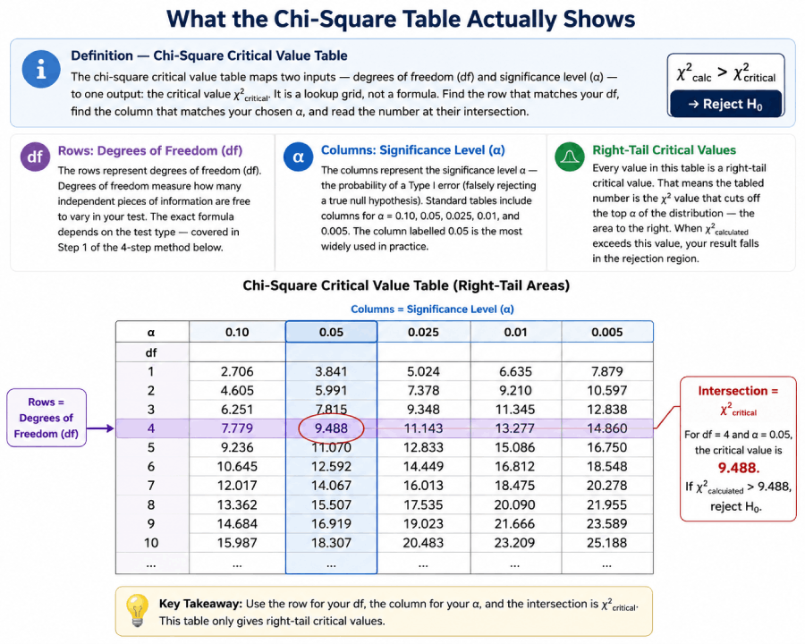
The rows represent degrees of freedom (df). Degrees of freedom measure how many independent pieces of information are free to vary in your test. The exact formula depends on the test type — covered in Step 1 of the 4-step method below.
The columns represent the significance level α — the probability of a Type I error (falsely rejecting a true null hypothesis). Standard tables include columns for α = 0.10, 0.05, 0.025, 0.01, and 0.005. The column labelled 0.05 is the most widely used in practice.
One detail that trips up many students: every value in this table is a right-tail critical value. That means the tabled number is the χ² value that cuts off the top α of the distribution — the area to the right. When χ²calculated exceeds this value, your result falls in the rejection region. For more on the chi-square distribution's shape and properties, see the full chi-square critical values table.
The 4-Step Method for Reading the Chi-Square Table
Step 1: Calculate df (goodness-of-fit: k−1; independence: (r−1)(c−1); variance: n−1). Step 2: Choose α (default 0.05). Step 3: Find the row for your df and the column for your α; read the intersection. Step 4: If χ²calc > critical value, reject H₀.
Step 1 — Calculate Your Degrees of Freedom
Degrees of freedom vary by test type. The formula you use depends on what kind of chi-square test you are running:
- Goodness-of-fit test: df = k − 1, where k is the number of categories. If you have 6 outcomes (like faces on a die), df = 6 − 1 = 5.
- Test of independence (contingency table): df = (r − 1)(c − 1), where r is the number of rows and c is the number of columns. A 2×3 table gives df = (2−1)(3−1) = 2.
- Variance test (one sample): df = n − 1, where n is the sample size. If n = 20, then df = 19.
A common mistake is using the wrong df formula — for example, applying k − 1 to a contingency table instead of (r−1)(c−1). This is Mistake 1 in the common mistakes section below. According to the National Institute of Standards and Technology's Engineering Statistics Handbook, getting the degrees of freedom right is the single most critical step in any chi-square test.
Step 2 — Choose Your Significance Level α
The significance level α is the maximum probability of a Type I error you are willing to accept — the chance of incorrectly rejecting a true null hypothesis. The default in most research fields is α = 0.05, meaning you accept a 5% chance of a false positive. A stricter test uses α = 0.01; a more lenient one uses α = 0.10.
The chi-square table columns correspond directly to these α values. If you choose α = 0.05, you will use the column labelled 0.05. This is the threshold below which your test result would occur by chance in a world where H₀ is true.
Step 3 — Find the Intersection
Navigate to the row matching your df and the column matching your α. The number at that intersection is χ²critical — the threshold your calculated statistic must exceed in order to reject the null hypothesis. The visual grid below shows this intersection for df = 5 and α = 0.05.
📍 Table Navigation Visual — df = 5, α = 0.05 → Critical Value = 11.071
Row: df = 5 (purple). Column: α = 0.05 (blue highlight). Intersection (purple cell): 11.071
Step 4 — Apply the Decision Rule
Compare your calculated test statistic (χ²calc) to the critical value you just looked up (χ²critical):
χ²_calc = your computed test statistic
χ²_critical = table lookup value
α = significance level (e.g., 0.05)
df = degrees of freedom
Rejecting H₀ means the observed data differ from what you would expect under the null hypothesis by more than chance alone can explain, at your chosen significance level. Failing to reject H₀ does not prove the null is true — it only means the data do not provide sufficient evidence against it. This is Mistake 4 in the common mistakes section, and it matters enormously for how you phrase conclusions.
Worked Example 1: Goodness-of-Fit Test (The Dice Problem)
The goodness-of-fit test is the most common entry point for chi-square. It asks: do observed frequencies match what a known theoretical distribution predicts? According to Rice University's open-access statistics textbook Introductory Statistics (OpenStax), this test requires only a single categorical variable and a hypothesized distribution — making it a staple of undergraduate courses and applied research alike.
You roll a six-sided die 60 times. If the die is fair, each face should appear 10 times. Observed counts: 8, 14, 9, 11, 7, 11. Is there evidence the die is biased?
State the hypotheses:
H₀: The die is fair — each face has probability 1/6.
H₁: The die is not fair — at least one face has a different probability.
Calculate the chi-square statistic using χ² = Σ(O − E)² / E:
| Face | Observed (O) | Expected (E) | (O − E) | (O − E)² | (O − E)² / E |
|---|---|---|---|---|---|
| 1 | 8 | 10 | −2 | 4 | 0.400 |
| 2 | 14 | 10 | +4 | 16 | 1.600 |
| 3 | 9 | 10 | −1 | 1 | 0.100 |
| 4 | 11 | 10 | +1 | 1 | 0.100 |
| 5 | 7 | 10 | −3 | 9 | 0.900 |
| 6 | 11 | 10 | +1 | 1 | 0.100 |
| χ²_calc = | 3.200 | ||||
Determine df and α: df = k − 1 = 6 − 1 = 5. Standard significance level: α = 0.05.
Look up the critical value: From the chi-square critical values table, row df = 5, column α = 0.05 → χ²critical = 11.071.
Apply the decision rule: χ²calc = 3.200. χ²critical = 11.071. Since 3.200 < 11.071, we fail to reject H₀.
✓ At the 5% significance level, there is insufficient evidence that the die is biased. The observed deviations (2 fewer 1s, 4 extra 2s, etc.) are well within the range expected by chance alone for a fair die rolled 60 times. To verify this calculation, use the chi-square calculator.
Worked Example 2: Test of Independence (Survey Data)
The chi-square test of independence determines whether two categorical variables are related, or whether they vary independently of each other. This is one of the most widely used statistical tests in social and behavioral science, described in detail in the Penn State STAT 500 course materials and the foundational textbook by Moore, McCabe & Craig.
200 people were surveyed on gender (male/female) and product preference (A/B/C). Is there a statistically significant relationship between gender and product preference?
State the hypotheses:
H₀: Gender and product preference are independent.
H₁: Gender and product preference are not independent (there is an association).
Observed frequencies (2×3 contingency table):
| Product A | Product B | Product C | Row Total | |
|---|---|---|---|---|
| Male | 40 | 30 | 50 | 120 |
| Female | 35 | 25 | 20 | 80 |
| Col Total | 75 | 55 | 70 | 200 |
Calculate expected frequencies using E = (row total × col total) / n:
| Cell | O | E = (row × col)/200 | (O−E)²/E |
|---|---|---|---|
| Male / A | 40 | (120×75)/200 = 45.0 | 0.556 |
| Male / B | 30 | (120×55)/200 = 33.0 | 0.273 |
| Male / C | 50 | (120×70)/200 = 42.0 | 1.524 |
| Female / A | 35 | (80×75)/200 = 30.0 | 0.833 |
| Female / B | 25 | (80×55)/200 = 22.0 | 0.409 |
| Female / C | 20 | (80×70)/200 = 28.0 | 2.286 |
| χ²_calc = | 5.881 | ||
Determine df: df = (r − 1)(c − 1) = (2 − 1)(3 − 1) = 1 × 2 = 2. Choose α = 0.05.
Navigate the table: Row df = 2, column α = 0.05 → χ²critical = 5.991. See the full chi-square table for reference.
Decision: χ²calc = 5.881 < χ²critical = 5.991. We fail to reject H₀, but only just barely. p is slightly above 0.05.
✓ At α = 0.05, there is not quite sufficient evidence to conclude that gender and product preference are related — though the result is borderline (χ² = 5.881 vs. critical value 5.991). For more worked examples including three-way tables, see hypothesis testing examples.
Worked Example 3: Variance Test (Two-Tailed Lookup)
Unlike the goodness-of-fit and independence tests — which are always right-tailed — a chi-square variance test can be one-tailed or two-tailed. The two-tailed version requires looking up two separate critical values from the table: one for each tail. This is the only chi-square context where you read two cells from the same df row.
A machine produces parts. The claimed variance is σ² = 4.0. A quality engineer takes n = 20 parts and finds a sample variance of s² = 5.3. Does the machine's variance differ significantly from the specification? (α = 0.05, two-tailed)
State the hypotheses:
H₀: σ² = 4.0 (variance equals specification)
H₁: σ² ≠ 4.0 (variance differs — two-tailed)
Calculate test statistic: χ² = (n − 1)s² / σ² = (19 × 5.3) / 4.0 = 100.7 / 4.0 = 25.175
Degrees of freedom: df = n − 1 = 20 − 1 = 19.
Two-tailed lookup at α = 0.05: Split α into two tails: α/2 = 0.025 per tail.
- Upper critical value (right tail, α/2 = 0.025): df = 19, column 0.025 → χ²upper = 32.852
- Lower critical value (left tail, α/2 = 0.025, uses column for 1 − α/2 = 0.975): df = 19, column 0.975 → χ²lower = 8.907
The rejection region is: χ² < 8.907 OR χ² > 32.852.
Decision: χ²calc = 25.175. Is 25.175 < 8.907 or > 32.852? No — 25.175 falls between the two critical values. Fail to reject H₀.
✓ At α = 0.05, there is insufficient evidence that the machine's variance differs from 4.0. A sample variance of 5.3 from n = 20 is within the range of variation expected for a machine with σ² = 4.0. Note that the two-tailed test requires reading both the 0.025 and 0.975 columns — a procedure described in the chi-square table reference section of this site.
How to Find the P-Value from the Table (Not Just the Critical Value)
Most students use the chi-square table only to find a critical value and make a binary reject/fail-to-reject decision. There is a second technique worth knowing: estimating a p-value range directly from the table, without a calculator.
The p-value approach works by finding which two column values your test statistic falls between, for a given df row. For example, with df = 5 and χ²calc = 9.80:
- From the table: column α = 0.10 gives 9.236; column α = 0.05 gives 11.071.
- Since 9.236 < 9.80 < 11.071, the p-value falls between 0.05 and 0.10.
- Conclusion: 0.05 < p < 0.10. You would fail to reject at α = 0.05 but reject at α = 0.10.
The key insight is that smaller α columns correspond to larger critical values. If your test statistic falls between two table values, your p-value falls between the corresponding α values for that row.
The table gives a p-value range (e.g., 0.025 < p < 0.05). For an exact p-value (e.g., p = 0.0318), use the chi-square calculator or a function like pchisq() in R or CHISQ.DIST.RT() in Excel. Always report exact values when publishing results.
The distinction between the p-value approach and the critical value approach is explained fully in our hypothesis testing guide. Both approaches give the same decision when you use them correctly.
4 Common Mistakes When Reading the Chi-Square Table
| # | Mistake | Correct Approach |
|---|---|---|
| 1 | Using df = k − 1 for a contingency table instead of (r−1)(c−1) | For any test with a two-way table, df = (rows − 1) × (columns − 1). For a 3×4 table: df = 2 × 3 = 6, not 3 or 11. |
| 2 | Reading the column header as the p-value ("I used the 0.05 column so p = 0.05") | The column is the significance level α — the threshold. The actual p-value is only equal to α if your test statistic exactly equals the critical value, which almost never happens. |
| 3 | Treating a small chi-square statistic as significant because "it's in the rejection region" | All chi-square tables use right-tail critical values. Significance means your statistic is larger than the critical value, not smaller. A chi-square statistic can never be negative. |
| 4 | Concluding "H₀ is true" after failing to reject it | Failing to reject H₀ means the data don't provide enough evidence against it. The null hypothesis could still be false — you just didn't have sufficient evidence or sample size to detect it. |
Quick Reference: Most-Used Critical Values
The table below covers the df values most commonly seen in introductory statistics. For all df values from 1 to 100 at five significance levels, see the full chi-square critical values table →
| df | α = 0.10 | α = 0.05 | α = 0.025 | α = 0.01 | α = 0.005 |
|---|---|---|---|---|---|
| 1 | 2.706 | 3.841 | 5.024 | 6.635 | 7.879 |
| 2 | 4.605 | 5.991 | 7.378 | 9.210 | 10.597 |
| 3 | 6.251 | 7.815 | 9.348 | 11.345 | 12.838 |
| 5 | 9.236 | 11.071 | 12.833 | 15.086 | 16.750 |
| 10 | 15.987 | 18.307 | 20.483 | 23.209 | 25.188 |
Need df values from 1–100? Download the chi-square table PDF for offline use, or bookmark the full interactive chi-square table.
Frequently Asked Questions
Chi-Square Table Reading — Cheat Sheet
| Concept | Formula / Value | When Used | Quick Note |
|---|---|---|---|
| Test Statistic | χ² = Σ(O − E)² / E | All chi-square tests | Every cell contributes independently |
| df — Goodness of Fit | k − 1 | One categorical variable vs. theory | k = number of categories |
| df — Independence | (r − 1)(c − 1) | Two-way contingency table | r = rows, c = columns |
| df — Variance Test | n − 1 | One-sample variance test | n = sample size |
| Decision Rule | χ²_calc > χ²_critical | All right-tailed tests | Reject H₀ if calc exceeds critical |
| Two-Tailed Variance | α/2 each tail | Testing σ² ≠ σ²₀ | Lookup 0.025 AND 0.975 columns |
| p-Value Range | Bracket between columns | When exact p-value not needed | "p is between 0.025 and 0.05" |
| Expected Cell Rule | E ≥ 5 per cell | Validating test assumptions | Small E invalidates chi-square |
Continue Learning at Statistics Fundamentals
Related Topics and Next Steps
Reading the chi-square table is one step in a broader hypothesis testing workflow. These guides cover the prerequisite and downstream concepts in natural reading order.
- Statistics Fundamentals — Return to the home page for the full topic index
- Chi-Square Critical Values Table (Full) — All df from 1–100 at five α levels, with distribution properties
- Chi-Square Test Guide — Full test procedure including assumptions, effect size (Cramér's V), and software output
- Hypothesis Testing — The complete framework: null hypothesis, α, p-values, Type I & II errors
- Hypothesis Testing Examples — More worked examples across test types
- ANOVA — The next step when comparing means across three or more groups
- Statistical Test Selector — Decision tree for choosing between chi-square, t-test, ANOVA, and more
- Chi-Square Calculator — Get exact p-values instantly without table lookup
- T-Distribution Table — Parallel reference for t-tests when comparing means
- Chi-Square Table PDF Download — Printable reference for exams and fieldwork
- NIST Engineering Statistics Handbook — Chi-Square Goodness-of-Fit — Authoritative federal reference for chi-square test procedures and assumptions
- OpenStax Introductory Statistics — Chapter 11: Chi-Square — Peer-reviewed open textbook used by hundreds of universities; freely accessible
- Yale University Department of Statistics — Chi-Square Tests — University course notes covering goodness-of-fit and independence tests with examples
- Khan Academy — Chi-Square Tests — Video walkthroughs and practice problems for students building intuition
- Penn State STAT 500 — Lesson 8: Chi-Square Tests — Graduate-level course notes from Penn State's Department of Statistics