Simple Linear Regression Calculator
Enter one X and Y pair per row, separated by a comma, space, or tab. You need at least 3 data pairs.
First calculate regression in the left tab, then enter any X value here to get the predicted Y. The equation ŷ = β₀ + β₁x is applied automatically.
What Is Simple Linear Regression?
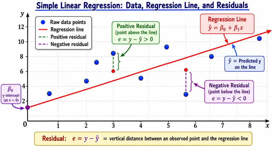
Simple linear regression is a method for modeling the straight-line relationship between one independent variable (X) and one continuous dependent variable (Y). The goal is to find the single line that minimizes the total squared distance between each observed data point and the line itself — a technique called ordinary least squares (OLS).
Think of how gas mileage drops as vehicle weight increases, or how monthly energy bills climb as winter temperatures fall. In both cases, one numeric variable reliably tracks another in a roughly straight-line pattern. Regression puts a precise mathematical equation on that pattern, so you can predict an unknown Y value from any given X. The resulting line is called the line of best fit, or the regression line.
According to the NIST/SEMATECH Engineering Statistics Handbook, linear regression is the most widely applied modeling technique in statistics because its outputs — slope, intercept, and R² — are interpretable without specialist training, yet the method underlies everything from econometric forecasts to clinical dose-response modeling.
The Simple Linear Regression Formula
The regression equation takes the form ŷ = β₀ + β₁x, where β₁ is the slope and β₀ is the y-intercept. Both are derived from your data using least squares formulas that no amount of eyeballing or guessing can match for accuracy.
Slope (β₁)
β₁ = [nΣXY − ΣX ⋅ ΣY]
     / [nΣX² − (ΣX)²]

n  = number of data pairs
XY = product of each pair
X² = square of each X value
Y-Intercept (β₀)
β₀ = (ΣY − β₁ΣX) / n

Equivalently:
β₀ = Ȳ − β₁X̄

X̄ = mean of X values
Ȳ = mean of Y values
Coefficient of Determination (R²)
R² = 1 − SSE / SST

SSE = Σ(Y − Ŷ)² (residuals SS)
SST = Σ(Y − Ȳ)² (total SS)
SSR = SST − SSE (regression SS)

Range: 0 ≤ R² ≤ 1
Pearson's Correlation (r)
r = [nΣXY − ΣXΣY]
 / √{[nΣX²−(ΣX)²][nΣY²−(ΣY)²]}

Range: −1 ≤ r ≤ +1
R² = r² (always)
sign(r) = sign(β₁)
The slope β₁ tells you how many units Y is expected to increase for each one-unit increase in X. A slope of 150 in a house-price model means each additional square foot is associated with $150 more in predicted price. The intercept β₀ is Y when X = 0 — sometimes interpretable (as a baseline cost), sometimes not (a house with zero square feet has no meaning, so β₀ is a mathematical anchor rather than a real prediction).
Step-by-Step Worked Example: Real Estate Pricing
Problem: A real estate analyst collects data on five properties. Does square footage (X) linearly predict sale price (Y)? Find the regression equation, R², and the predicted price for a 1,900 sq ft home.
The dataset below maps square footage to sale price. You can load this exact example into the calculator above using the "Example (Real Estate)" button.
| Property | X (sq ft) | Y (Price $) | X² | XY | Ŷ (Predicted) | Residual e |
|---|---|---|---|---|---|---|
| House 1 | 1,200 | 200,000 | 1,440,000 | 240,000,000 | 197,500 | +2,500 |
| House 2 | 1,500 | 245,000 | 2,250,000 | 367,500,000 | 242,500 | +2,500 |
| House 3 | 1,800 | 290,000 | 3,240,000 | 522,000,000 | 287,500 | +2,500 |
| House 4 | 2,100 | 335,000 | 4,410,000 | 703,500,000 | 332,500 | +2,500 |
| House 5 | 2,400 | 380,000 | 5,760,000 | 912,000,000 | 377,500 | +2,500 |
| Totals | 9,000 | 1,450,000 | 17,100,000 | 2,745,000,000 | — | — |
n = 5, ΣX = 9,000, ΣY = 1,450,000, ΣX² = 17,100,000, ΣXY = 2,745,000,000
β₁ = [5 × 2,745,000,000 − 9,000 × 1,450,000] / [5 × 17,100,000 − 9,000²]
= [13,725,000,000 − 13,050,000,000] / [85,500,000 − 81,000,000]
= 675,000,000 / 4,500,000 = 150
X̄ = 9,000 / 5 = 1,800 Ȳ = 1,450,000 / 5 = 290,000
β₀ = Ȳ − β₁ ⋅ X̄ = 290,000 − 150 × 1,800 = 290,000 − 270,000 = 20,000
ŷ = 20,000 + 150x
Each additional square foot adds $150 to predicted price, with a baseline of $20,000.
SST = (200,000−290,000)² + (245,000−290,000)² + … = 28,250,000,000
SSE = 2,500² × 5 = 31,250,000
R² = 1 − 31,250,000 / 28,250,000,000 ≈ 0.9989
ŷ = 20,000 + 150 × 1,900 = 20,000 + 285,000 = $305,000
Result: Regression equation is ŷ = 20,000 + 150x. R² = 0.9989 means square footage explains 99.89% of the variance in price — a near-perfect linear fit in this small, uniform dataset. A 1,900 sq ft home is predicted to sell for $305,000. Use the "Example (Real Estate)" button in the calculator above to verify each step.
Interpreting Your Results: R², Pearson's r, and Residuals
Three outputs carry most of the interpretive weight in a simple linear regression: the equation itself, R², and the residual pattern. Getting all three right is what separates a useful model from a misleading one.
| Metric | Formula | What It Measures | Interpretation Guide |
|---|---|---|---|
| Regression Equation | ŷ = β₀ + β₁x | Predicts Y from any X value | β₁ is the change in Y per unit of X; β₀ is Y when X = 0 |
| Slope (β₁) | (nΣXY−ΣXΣY) / (nΣX²−(ΣX)²) | Rate of change in Y per unit X | Positive = Y rises as X rises; Negative = inverse relationship |
| Y-Intercept (β₀) | Ȳ − β₁X̄ | Predicted Y when X = 0 | May not be meaningful if X = 0 is outside the data range |
| R² | 1 − SSE/SST | Proportion of Y variance explained by X | 0 = no fit; 1 = perfect fit; context determines what is "good" |
| Pearson's r | √R² ⋅ sign(β₁) | Strength and direction of linear association | |r| > 0.7 = strong; 0.4–0.7 = moderate; <0.4 = weak |
| Residual (e) | Y − Ŷ | Prediction error for each observation | Should be random; patterns suggest violated assumptions |
| SSE | Σ(Y−Ŷ)² | Total unexplained variation | Lower is better; used to calculate R² and standard error |
| SST | Σ(Y−Ȳ)² | Total variation in Y | Baseline; SSR + SSE always equals SST |
Difference Between r and R²
Pearson's r and R² both measure model fit, but they serve different questions. An r of +0.91 tells you the relationship is strong and positive. R² = 0.83 (which is 0.91²) tells you the model accounts for 83% of the variance in Y — leaving 17% unexplained by X. In simple linear regression these two always relate by R² = r². In multiple regression, R² still works the same way but r no longer applies the same connection.
Assumptions of Simple Linear Regression (LINE)
Regression results are only trustworthy when the four assumptions hold. Statisticians use the acronym LINE to remember them. Violating these doesn't always break the model — but it does change which conclusions you can draw.
The relationship between X and Y is linear — a straight line accurately represents the pattern. Check with a scatter plot before running regression. If the cloud of points curves, a linear model will miss the shape of the data.
Observations are independent of one another. Violated in time-series data (today's value depends on yesterday's) and in clustered samples. Independence cannot be checked from the data alone — it depends on your study design.
The residuals — not the raw data — are approximately normally distributed. This matters most for small samples when using the model for inference (confidence intervals, p-values). Large samples are robust by the Central Limit Theorem.
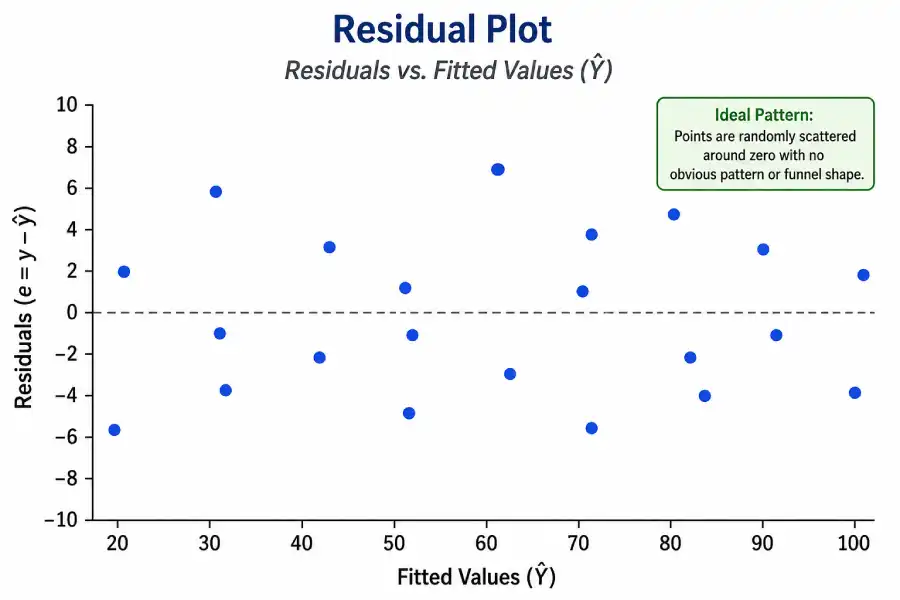
Residual variance stays constant across all X values. A funnel shape in a residual plot — where scatter fans out as X increases — signals heteroscedasticity. Weighted least squares or log-transformation often fixes this.
Penn State's STAT 501 course, available via online.stat.psu.edu, provides a thorough walkthrough of diagnosing each assumption using residual plots, Q-Q plots, and the Durbin-Watson test for independence. Their materials are widely cited in applied statistics curricula for good reason — the worked examples track industrial and biological datasets where at least one assumption is always slightly bent.
Simple Linear Regression in Python, Excel, and R
For analysts working with larger datasets, the following code snippets replicate exactly what this calculator computes — useful for verifying outputs before integrating regression into a larger workflow.
Python (NumPy / SciPy / Scikit-Learn)
import numpy as np
from scipy import stats

x = np.array([1200, 1500, 1800, 2100, 2400])
y = np.array([200000, 245000, 290000, 335000, 380000])

slope, intercept, r, p_value, std_err = stats.linregress(x, y)

print(f"Slope (β₁):     {slope:.4f}")        # 150.0
print(f"Intercept (β₀): {intercept:.4f}")    # 20000.0
print(f"R² value:       {r**2:.4f}")         # 0.9989
print(f"Pearson r:      {r:.4f}")            # 0.9994
print(f"Predicted (1900 sqft): {intercept + slope * 1900:.0f}")  # 305000
Microsoft Excel (LINEST function)
=LINEST(B2:B6, A2:A6, TRUE, TRUE)   // Returns full stats array: slope, intercept, R², etc.

// Individual outputs:
=SLOPE(B2:B6, A2:A6)               // Slope β₁  → 150
=INTERCEPT(B2:B6, A2:A6)           // Intercept β₀ → 20000
=RSQ(B2:B6, A2:A6)                 // R² → 0.9989
=CORREL(A2:A6, B2:B6)              // Pearson r → 0.9994
=FORECAST.LINEAR(1900, B2:B6, A2:A6)  // Predicted Y → 305000
Note: Excel's LINEST vs. this calculator agrees to all decimal places on slope and intercept. The calculator above vs. =LINEST() is a useful cross-check students can run side by side for any homework dataset.
R
x <- c(1200, 1500, 1800, 2100, 2400)
y <- c(200000, 245000, 290000, 335000, 380000)

model <- lm(y ~ x)
summary(model)
# Coefficients: (Intercept) = 20000, x = 150
# R-squared: 0.9989

predict(model, newdata = data.frame(x = 1900))  # 305000
plot(x, y); abline(model, col = "blue")         # Scatter + regression line
Simple vs. Multiple Linear Regression: When to Use Which
The choice between simple and multiple regression comes down to how many independent variables you need to describe reality accurately. Simple regression works when one predictor genuinely captures most of the variation. Once a second variable adds meaningful explanatory power — and is not just noise — multiple regression is the appropriate extension.
| Feature | Simple Linear Regression | Multiple Linear Regression |
|---|---|---|
| Predictors | One (X) | Two or more (X₁, X₂, …) |
| Equation | ŷ = β₀ + β₁x | ŷ = β₀ + β₁x₁ + β₂x₂ + … |
| Slope interpretation | Change in Y per unit X | Change in Y per unit X₆ holding all other X constant |
| Fit metric | R² | Adjusted R² (penalizes extra predictors) |
| Typical use | Initial exploration; one clear driver | Real-world prediction where multiple factors matter |
| New risk | Omitted variable bias | Multicollinearity between predictors |
For a full treatment of extending the model beyond one predictor, see the multiple linear regression guide on this site. When your outcome is categorical rather than continuous, logistic regression is the standard choice — it models the log-odds of a binary event rather than a continuous Y.
Related Topics on Statistics Fundamentals
Linear regression connects to probability, hypothesis testing, and visualization. These pages build the surrounding foundation.
Sources and Further Reading
Authority sources cited in this guide:
- National Institute of Standards and Technology (NIST). NIST/SEMATECH e-Handbook of Statistical Methods — Linear Least Squares Regression. itl.nist.gov
- Penn State Eberly College of Science. STAT 501: Regression Methods — Lesson 1: Simple Linear Regression. online.stat.psu.edu
- UCLA Institute for Digital Research and Education. Introduction to Linear Regression Analysis. stats.oarc.ucla.edu
- MIT OpenCourseWare. 18.650 Statistics for Applications — Regression Models. ocw.mit.edu
- Montgomery, D.C., Peck, E.A., & Vining, G.G. Introduction to Linear Regression Analysis, 5th ed. Wiley, 2012.
- Wikipedia contributors. Simple linear regression. en.wikipedia.org
Frequently Asked Questions
The regression equation is ŷ = β₀ + β₁x. The slope is β₁ = [nΣXY − ΣXΣY] / [nΣX² − (ΣX)²] and the y-intercept is β₀ = Ȳ − β₁X̄. Both are derived from your data using the least squares method, which minimizes the sum of squared residuals between observed Y values and the regression line.
R² (the coefficient of determination) is the proportion of total variance in Y that the regression model explains. An R² of 0.85 means 85% of the spread in Y is accounted for by X alone; the remaining 15% is unexplained variation. R² ranges from 0 to 1. Whether a given value is "good" depends on context — physical sciences often see R² above 0.95, while social science models with R² of 0.40 can still be valuable.
Pearson's r is the correlation coefficient — it ranges from −1 to +1 and captures both the strength and direction of the linear relationship. R² is simply r squared (always positive) and tells you the fraction of variance explained. An r of −0.90 means a strong negative relationship; its R² = 0.81 means the model explains 81% of variance regardless of direction. In simple linear regression, R² = r² exactly. In multiple regression, R² extends naturally but r no longer applies the same way.
A residual is the vertical gap between an observed data point and the regression line: e = Y − Ŷ. Points above the line have positive residuals; points below have negative ones. The least squares method minimizes Σe² — the sum of all squared residuals — which is why it produces the best possible straight-line fit. Examining residuals after fitting is essential: patterns (curves, funnels, clusters) mean the linear model isn't capturing all the structure in your data.
The four assumptions (LINE): Linearity — Y and X have a linear relationship, visible in a scatter plot; Independence — observations don't depend on each other (violated in time-series without correction); Normality — residuals are approximately normally distributed (test with a Q-Q plot); Equal variance / Homoscedasticity — residual spread is constant across all X values (a funnel pattern in a residual plot signals a problem). Violating these doesn't always invalidate the model but does limit which inferences you can trust.
Simple linear regression uses one predictor variable: ŷ = β₀ + β₁x. Multiple linear regression uses two or more: ŷ = β₀ + β₁x₁ + β₂x₂ + …. In multiple regression, each slope β₆ represents the effect of that variable while holding all other predictors constant — which changes the interpretation substantially. See the multiple linear regression guide for the full extension with adjusted R² and F-test details.
Outliers at the extremes of X — points with high leverage — can pull the regression line toward them and substantially change the slope. A single high-leverage outlier can inflate R² (making the model look better than it is) or deflate it, depending on where the point falls relative to the true trend. Always examine the scatter plot and residuals table before trusting the model. If a genuine data error is found, remove or correct it. If the outlier is a real observation, consider reporting results with and without it.
No. Regression reveals statistical association — not causation. A high R² means X is a reliable predictor of Y in the observed data, but the causal mechanism could run the other direction, both variables might respond to a third confounding variable, or the pattern could be coincidental. Establishing causation requires either a controlled experiment with random assignment or a well-designed natural experiment. This is why researchers carefully distinguish "X predicts Y" from "X causes Y" when reporting regression findings.