What Is Logistic Regression?
Despite containing the word "regression," logistic regression is a classification algorithm. The name reflects its origins in statistical modeling, not its function. What it produces is not a continuous prediction but a probability — a number between 0 and 1. A threshold (typically 0.5) then converts that probability into a class label: above the threshold means class 1 (positive), below means class 0 (negative).
The algorithm belongs to the family of generalized linear models. It extends ordinary linear regression to classification by transforming the linear predictor through the logistic function. This makes it one of the most interpretable machine learning models available — a quality that has kept it relevant across medicine, finance, social science, and engineering for over 70 years. According to foundational work in this area, the logistic regression model was formalized by David Cox in 1958 in the Journal of the Royal Statistical Society, building on earlier probability modeling by Joseph Berkson in the 1940s.
One-Paragraph Beginner Definition
Logistic regression is a method used to predict whether something belongs to one of two groups — for example, whether a patient has a disease (yes/no) or whether an email is spam (yes/no). It works by calculating the probability of each outcome using a mathematical function called the sigmoid curve, which squashes any number into a value between 0 and 1. If the predicted probability exceeds 0.5, the model classifies the observation as class 1 (positive); otherwise it predicts class 0. Despite its name, logistic regression is a classification algorithm, not a regression algorithm.
Key Characteristics of Logistic Regression
- Type: Supervised learning, binary classification (extensions exist for multi-class)
- Output: Probability in (0, 1); then class label via threshold
- Core function: Sigmoid σ(z) = 1 / (1 + e−z)
- Estimation: Maximum Likelihood Estimation (MLE), not Ordinary Least Squares
- Interpretability: High — coefficients map directly to log-odds and odds ratios
- Regularization: L1 (LASSO) and L2 (Ridge) variants available for high-dimensional data
- Baseline rule: Use logistic regression before trying complex models — if it performs well, the interpretability benefit is substantial
The Logistic Regression Formula Explained
The complete logistic regression model involves three mathematically equivalent representations: the probability form, the log-odds (logit) form, and the odds ratio form. Each has a specific use case in analysis and interpretation. Understanding all three is essential for reading model output correctly.
The Logistic (Sigmoid) Function
σ(z) = probability output in (0, 1)
e = Euler's number ≈ 2.71828
z = linear combination of features
The sigmoid function was chosen for logistic regression because it has three ideal properties for binary classification: it is bounded between 0 and 1 for all real inputs, it is smooth and differentiable everywhere (required for gradient-based optimization), and it has a natural interpretation as a probability. When z → +∞, σ(z) → 1. When z → −∞, σ(z) → 0. At z = 0, σ(z) = 0.5 exactly — this is the decision boundary.
Sigmoid Curve — Shape, Range, and Decision Boundary
The S-shaped sigmoid curve maps the linear predictor z to a probability. When z = 0, P = 0.5 — the decision boundary. The curve asymptotes to 0 and 1 but never reaches them.
Log-Odds and Probability Interpretation
Logistic regression is linear in log-odds space. The model estimates a linear function of the predictors, then exponentiates it and rescales through the sigmoid to get a probability. This means that while the probability curve is S-shaped and nonlinear, the underlying relationship being modeled is linear when expressed as log-odds. This distinction is critical for correct interpretation: a one-unit increase in X₁ increases the log-odds by β₁ — not the probability directly.
| Symbol | Name | Plain-Language Definition | Range |
|---|---|---|---|
| P(Y=1) | Predicted Probability | The estimated probability that the outcome is class 1. What the model outputs. | (0, 1) |
| β₀ | Intercept | Log-odds of Y=1 when all predictors equal zero. Not always meaningful on its own. | (−∞, +∞) |
| β₁…βₙ | Coefficients | Change in log-odds for a one-unit increase in the corresponding predictor, holding others constant. | (−∞, +∞) |
| X₁…Xₙ | Predictor Variables (Features) | The input variables used to predict the outcome. Can be continuous or dummy-coded categorical. | Varies |
| e | Euler's Number | The base of the natural logarithm, approximately 2.71828. Used in the sigmoid and odds ratio calculations. | ≈ 2.718 |
| eβ | Odds Ratio | The multiplicative change in odds of Y=1 per one-unit increase in a predictor. The primary interpretation tool. | (0, +∞) |
Odds Ratio Explained with Examples
The odds ratio is the most practical output from a logistic regression model. It translates the abstract coefficient β into a concrete, multiplicative statement about how each predictor affects the outcome.
OR = eβ. If OR = 2.0 → the odds of Y=1 double for each one-unit increase in X. If OR = 0.5 → the odds are halved. If OR = 1.0 → X has no effect on the outcome. OR > 1 means X increases the probability; OR < 1 means X decreases it.
Worked example: A logistic regression model predicts diabetes from fasting blood glucose level. The coefficient for glucose is β = 0.035. So OR = e0.035 = 1.036. This means a one-unit (mg/dL) increase in fasting glucose increases the odds of diabetes by 3.6%. A 50 mg/dL increase would multiply the odds by e0.035 × 50 = e1.75 ≈ 5.75 — nearly a six-fold increase in odds.
Maximum Likelihood Estimation (MLE)
yᵢ = observed class (0 or 1)
p̂ᵢ = predicted probability for observation i
Σ = sum over all n observations
Unlike linear regression, which minimizes the sum of squared errors (OLS), logistic regression maximizes the log-likelihood function above. This function penalizes confident wrong predictions severely: predicting p̂ = 0.99 for a true negative (y = 0) results in log(1 − 0.99) = log(0.01) ≈ −4.6, a large negative contribution to the total. The model adjusts β values through an iterative optimization algorithm until the log-likelihood can no longer be increased. This is why logistic regression has no closed-form solution and requires iterative computation, as documented in the Penn State STAT 415 course materials.
When Should You Use Logistic Regression?
Binary Outcome Requirement
The fundamental requirement for standard logistic regression is a binary dependent variable: an outcome that takes exactly two values, conventionally coded as 0 (negative class) and 1 (positive class). Examples include survived/died, purchased/did not purchase, diseased/healthy, approved/denied. If the outcome has more than two categories, multinomial or ordinal logistic regression is required.
| Use Logistic Regression When | Do NOT Use — Alternative Instead |
|---|---|
| Outcome is binary (0/1, yes/no) | Outcome is continuous → use linear regression |
| Need probability output + interpretation | Outcome has 3+ unordered categories → use multinomial LR |
| Need to quantify each predictor's effect | Outcome has ordinal categories → use ordinal LR |
| Small-to-medium dataset, speed matters | Complex nonlinear interactions dominate → try tree-based models |
| Regulatory/legal explainability required | Very high-dimensional sparse data → use regularized LR or SVM |
| Use as a baseline model before complex methods | Count data as outcome → use Poisson regression |
The 5 Key Assumptions of Logistic Regression
Violating these assumptions does not prevent the model from running — it runs regardless. What it prevents is valid inference. Following the standard set out in Hosmer, Lemeshow, and Sturdivant's Applied Logistic Regression (3rd ed., Wiley, 2013) — the definitive academic reference on this topic — the five assumptions are:
Binary (or Ordinal) Dependent Variable
The outcome variable must be categorical, not continuous. Standard logistic regression requires exactly two outcome categories. If it has 3+ categories, the mathematical machinery of the binary model breaks down.
Independence of Observations
Observations must be independent of each other. Repeated measures on the same subject, time-series data, or clustered data (students in schools) violate this assumption. Use mixed-effects logistic regression for clustered data.
No Severe Multicollinearity
Predictor variables should not be highly correlated with each other. Severe multicollinearity inflates standard errors, making coefficient estimates unstable and p-values unreliable. Check with Variance Inflation Factors (VIF < 10).
Linearity of Log-Odds
Continuous predictors must have a linear relationship with the log-odds of the outcome — not with the probability directly. Check using the Box-Tidwell test or by plotting log-odds against each continuous predictor.
Adequate Sample Size
The rule of thumb, established in simulation studies (Peduzzi et al., 1996, Journal of Clinical Epidemiology), is at least 10 events per predictor variable (EPV ≥ 10). With 5 predictors and an outcome with 30% positive cases, you need at least 5 × 10 / 0.30 ≈ 167 observations minimum.
Step-by-Step Logistic Regression Tutorial
The following six-step workflow follows the standard academic and practitioner pipeline. Steps reference Python implementations using scikit-learn, which the scikit-learn documentation defines as one of the most widely used logistic regression libraries.
Step 1 — Define the Binary Outcome Variable
Before writing any code, precisely define what Y=1 and Y=0 mean. "Customer churned in the next 30 days" is a well-defined outcome. "Customer was dissatisfied" is not — it requires a measurement instrument. Lock down the definition before data collection to avoid outcome definition drift.
Step 2 — Explore and Prepare Your Data
Check for missing values, extreme outliers, and class imbalance. A dataset with 95% class 0 and 5% class 1 will produce a model that predicts class 0 for almost everything and still achieves 95% accuracy — a deceptive result. Address imbalance through stratified train/test splits, oversampling (SMOTE), undersampling, or class weights.
Step 3 — Select Features and Check Multicollinearity
Remove features with near-zero variance and those with VIF > 10 (or VIF > 5 for stricter standards). Encode categorical variables using dummy coding (one-hot encoding minus one column to avoid the dummy variable trap). Scale continuous features with standardization if using regularized logistic regression.
Step 4 — Train the Model (Python / R Examples)
from sklearn.linear_model import LogisticRegression
from sklearn.model_selection import train_test_split
from sklearn.preprocessing import StandardScaler
import pandas as pd
# Step 3: Split data (stratify preserves class balance)
X_train, X_test, y_train, y_test = train_test_split(
X, y, test_size=0.2, random_state=42, stratify=y
)
# Step 4: Scale features (important for regularized LR)
scaler = StandardScaler()
X_train_sc = scaler.fit_transform(X_train)
X_test_sc = scaler.transform(X_test)
# Step 4: Fit model (C=1/λ — higher C = less regularization)
model = LogisticRegression(C=1.0, solver='lbfgs', max_iter=1000)
model.fit(X_train_sc, y_train)
# Step 5: Probabilities and predictions
y_prob = model.predict_proba(X_test_sc)[:, 1] # P(Y=1)
y_pred = model.predict(X_test_sc) # class label at 0.5
# Coefficients → odds ratios
import numpy as np
odds_ratios = np.exp(model.coef_[0])
coef_df = pd.DataFrame({
'Feature': X.columns,
'Coefficient': model.coef_[0],
'Odds Ratio': odds_ratios
})
print(coef_df.sort_values('Odds Ratio', ascending=False))
Step 5 — Interpret the Output and Coefficients
Print the coefficient table with odds ratios. For each feature, determine: (a) sign of β (positive = increases probability, negative = decreases), (b) magnitude of eβ (far from 1.0 = strong effect), and (c) p-value or confidence interval to assess statistical significance. Statsmodels provides full statistical output for Python; use glm() in R for the equivalent.
Step 6 — Evaluate with Confusion Matrix, ROC-AUC, F1
Never evaluate a binary classifier on accuracy alone, especially with class imbalance. Use the full evaluation suite described in Section 8 of this guide. The standard reference for evaluation metrics is the Fawcett (2006) ROC analysis tutorial, published in Pattern Recognition Letters, which defines AUC as the standard threshold-independent measure of classifier discrimination.
Worked Examples of Logistic Regression
Example 1 — Predicting Customer Churn
A telecom company wants to predict whether a customer will cancel their subscription within 30 days. Features include: monthly charges ($75), tenure (12 months), number of support tickets (3), and contract type (month-to-month = 1).
Model equation: log-odds(churn) = −3.2 + 0.021(charges) − 0.045(tenure) + 0.38(tickets) + 1.12(month-to-month)
Compute z: z = −3.2 + 0.021(75) − 0.045(12) + 0.38(3) + 1.12(1) = −3.2 + 1.575 − 0.54 + 1.14 + 1.12 = 0.095
Apply sigmoid: P(churn) = 1 / (1 + e−0.095) = 1 / (1 + 0.909) = 0.524 (52.4% chance of churn)
Decision at threshold 0.5: 0.524 > 0.5 → Predict: Churn (class 1)
Odds ratio interpretation: Contract type OR = e1.12 = 3.06 — month-to-month customers are over 3× more likely to churn than long-term contract customers, holding other factors constant.
✓ Customer predicted to churn. High monthly charges + month-to-month contract are the primary risk drivers. Action: proactive retention offer targeting customers with OR-dominant features.
Example 2 — Disease Diagnosis (Diabetes Dataset)
Using the Pima Indians Diabetes Dataset (UCI Repository), predict diabetes from: glucose (148 mg/dL), BMI (33.6), age (50), and number of pregnancies (1). This dataset was used in a seminal 1988 machine learning benchmark study by Smith et al.
Model coefficients (trained on full dataset): β₀ = −8.4, β_glucose = 0.038, β_BMI = 0.071, β_age = 0.015, β_pregnancies = 0.122
Compute z: z = −8.4 + 0.038(148) + 0.071(33.6) + 0.015(50) + 0.122(1) = −8.4 + 5.624 + 2.386 + 0.75 + 0.122 = 0.482
Apply sigmoid: P(diabetes) = 1 / (1 + e−0.482) = 0.618 (61.8% probability of positive diagnosis)
Note on threshold: In medical screening, a lower threshold (e.g., 0.3) may be preferred to maximize recall (sensitivity), catching more true positives at the cost of more false positives. This is a clinical decision, not a statistical one.
✓ Predicted diabetic at default threshold. The glucose level is the dominant driver (OR = e0.038×148 contribution is substantial). Clinical applications should use domain-specific threshold calibration.
Example 3 — Email Spam Classification
In text classification for spam detection, logistic regression operates on TF-IDF feature vectors. Each word becomes a predictor; the coefficient for that word represents how strongly its presence predicts spam vs. legitimate mail. Words like "free," "click here," and "guaranteed" get large positive coefficients. Words like "invoice," "meeting," and "attached" get negative coefficients. Because logistic regression is linear, it handles high-dimensional sparse text data efficiently — often matching or exceeding more complex models on well-curated datasets.
Example 4 — Credit Approval / Scoring
Credit scoring is one of the oldest applications of logistic regression, with formal adoption in lending starting in the 1960s. The output probability P(default) is scaled to a credit score. Under the Equal Credit Opportunity Act and Basel banking regulations, lenders must provide "adverse action notices" — specific reasons a loan was denied. Logistic regression's coefficient interpretability makes this legally compliant; a black-box model cannot satisfy this requirement. Each applicant's score is a direct function of their feature values and the model's coefficients.
Example 5 — Student Pass/Fail Prediction
A university uses logistic regression to predict first-year student outcomes: P(fail) from hours studied per week, attendance rate, prior GPA, and financial aid status. A student with 8 hours/week, 75% attendance, 2.8 prior GPA, and no financial aid might get P(fail) = 0.34 — below threshold at 0.5, so predicted to pass. This is used for early intervention programs: students above a lower threshold (e.g., 0.25) are contacted by academic advisors. The interpretable model lets advisors explain exactly which factors elevate the risk score, making interventions specific and actionable.
How to Interpret Logistic Regression Output
Reading Coefficients (β Values)
Raw coefficients from logistic regression output are in log-odds units. A coefficient of β = 0.7 means a one-unit increase in X increases the log-odds of Y=1 by 0.7. This is rarely interpretable on its own. Exponentiate to get the odds ratio: e0.7 = 2.01. Now the interpretation is clear: a one-unit increase in X doubles the odds of the positive outcome.
| Coefficient (β) | Odds Ratio (eβ) | Plain-Language Interpretation |
|---|---|---|
| −0.693 | 0.50 | One-unit increase in X halves the odds of Y=1 |
| 0 | 1.00 | X has no effect on the outcome |
| 0.405 | 1.50 | One-unit increase increases odds by 50% |
| 0.693 | 2.00 | One-unit increase doubles the odds |
| 1.099 | 3.00 | One-unit increase triples the odds |
| 2.303 | 10.00 | One-unit increase increases odds tenfold |
p-Values and Statistical Significance
Each coefficient comes with a Wald statistic and p-value testing H₀: β = 0 (the predictor has no effect). A p-value below 0.05 indicates the coefficient is statistically significantly different from zero at the 5% level. However — as with all significance testing — statistical significance does not imply practical importance. A p < 0.001 on a predictor with OR = 1.02 may be statistically "real" but practically negligible. Always report effect sizes alongside p-values, consistent with the American Statistical Association's 2016 Statement on P-Values.
Pseudo R-Squared (McFadden's R²)
Logistic regression has no direct equivalent to the R² from linear regression. McFadden's pseudo R² = 1 − (log-likelihood of full model / log-likelihood of null model). Values between 0.2 and 0.4 are generally considered good fit in logistic regression, according to McFadden's original 1974 paper. Unlike linear R², it does not represent "variance explained" — it is a likelihood ratio statistic scaled to (0, 1).
Visual Explanations
Decision Boundary in 2D Feature Space
Decision Boundary — 2D Feature Space (Two Predictors)
The dashed line is the decision boundary where P(Y=1) = 0.5 exactly, i.e., where β₀ + β₁X₁ + β₂X₂ = 0. Logistic regression produces a linear boundary in feature space.
Confusion Matrix (TP, FP, TN, FN)
Confusion Matrix — 2×2 Classification Results
TP = model correctly predicted positive. TN = correctly predicted negative. FP = predicted positive when actually negative (Type I). FN = predicted negative when actually positive (Type II — often the more costly error in medical/fraud contexts).
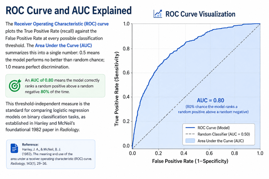
ROC Curve and AUC Explained
The Receiver Operating Characteristic (ROC) curve plots the True Positive Rate (recall) against the False Positive Rate at every possible classification threshold. The Area Under the Curve (AUC) summarizes this into a single number: 0.5 means the model performs no better than random chance; 1.0 means perfect discrimination. An AUC of 0.80 means the model correctly ranks a random positive above a random negative 80% of the time. This threshold-independent measure is the standard for comparing logistic regression models on binary classification tasks, as established in Hanley and McNeil's foundational 1982 paper in Radiology.
Model Evaluation Metrics
The confusion matrix provides the raw counts from which all standard binary classification metrics are derived. Using the notation TP (true positives), FP (false positives), TN (true negatives), FN (false negatives):
| Metric | Formula | What It Measures | When to Prioritize |
|---|---|---|---|
| Accuracy | (TP + TN) / Total | Overall correct predictions | Only with balanced classes |
| Precision | TP / (TP + FP) | Of predicted positives, what fraction are correct | When FP cost is high (spam filter) |
| Recall (Sensitivity) | TP / (TP + FN) | Of actual positives, what fraction were caught | When FN cost is high (disease screening) |
| Specificity | TN / (TN + FP) | Of actual negatives, what fraction were correctly identified | Paired with sensitivity in medical tests |
| F1 Score | 2 × (Precision × Recall) / (Precision + Recall) | Harmonic mean of precision and recall | Imbalanced classes, balanced FP/FN cost |
| ROC-AUC | Area under ROC curve | Threshold-independent discriminative ability | Comparing models; imbalanced datasets |
| McFadden R² | 1 − (LL_full / LL_null) | Goodness-of-fit; likelihood ratio relative to null | Model comparison, goodness of fit |
Logistic Regression Probability Calculator
🧮 Sigmoid / Logistic Regression Probability Calculator
Enter the linear combination z = β₀ + β₁X₁ + … (the weighted sum of your coefficients and feature values). The calculator outputs P(Y=1) from the sigmoid function.
Logistic Regression vs. Other Methods
Logistic Regression vs. Linear Regression
| Property | Logistic Regression | Linear Regression |
|---|---|---|
| Outcome type | Binary categorical (0/1) | Continuous (any real number) |
| Output range | (0, 1) — probability | (−∞, +∞) — unbounded |
| Estimation method | Maximum Likelihood (MLE) | Ordinary Least Squares (OLS) |
| Loss function | Log-loss (cross-entropy) | Mean Squared Error (MSE) |
| Error distribution | Binomial — no normality required | Assumes normally distributed errors |
| Interpretation unit | Log-odds / Odds Ratio | Direct units (e.g., dollars, cm) |
| Goodness of fit | McFadden R², AUC | R² (variance explained) |
Logistic Regression vs. Decision Trees
Decision trees partition the feature space into rectangular regions using if/then splits. They naturally capture nonlinear relationships and feature interactions without explicit specification. Logistic regression fits a single linear decision boundary and requires manual feature engineering for nonlinear relationships. Trees are harder to interpret at depth; logistic regression produces globally interpretable coefficients. For small-to-medium datasets with mostly linear relationships, logistic regression typically outperforms decision trees. As dataset complexity increases, tree-based ensembles (random forest, gradient boosting) often dominate.
Logistic Regression vs. Random Forest
Random forest combines hundreds of decision trees and captures complex nonlinear relationships that logistic regression misses. In exchange, it loses coefficient interpretability and requires more compute. On tabular data benchmarks, logistic regression is typically competitive when the true relationship is approximately linear in log-odds. A common practice: fit logistic regression first as a baseline; if the gap to random forest is small (<2–3% AUC), prefer logistic regression for interpretability and deployability.
Binary vs. Multinomial Logistic Regression
Binary logistic regression models P(Y=1) for a two-class outcome. Multinomial logistic regression (also called softmax regression) extends this to k classes by fitting k-1 separate log-odds equations using one class as the reference. Each equation compares one class against the reference; together they produce a probability distribution over all k classes that sums to 1.
Real-World Applications
Healthcare and Disease Prediction
Logistic regression has been the primary model in clinical prediction rules for decades. The Framingham Heart Study (Dawber et al., 1951) pioneered the use of logistic regression to predict cardiovascular disease risk from risk factors including age, blood pressure, cholesterol, and smoking status. The resulting Framingham Risk Score is still in clinical use today, demonstrating the model's durability when assumptions are met. Medical applications require interpretability not just for clinical understanding, but because regulatory bodies like the FDA require explainable models for clinical decision support software.
Credit Scoring and Fraud Detection
Credit scoring was one of the earliest commercial applications of logistic regression, predating modern machine learning by decades. Fair Isaac Corporation (FICO) developed the first automated credit scoring system in 1958 using what is now recognizable as logistic regression methodology. In fraud detection, logistic regression provides the interpretable output needed to justify blocking a transaction — essential for customer service and regulatory compliance under the Payment Services Directive (PSD2) in the EU.
Marketing Analytics and Conversion Modeling
In digital marketing, logistic regression models predict P(conversion | user features + context). The model's coefficient for "email campaign" might show OR = 2.3, meaning email-exposed users are 2.3× more likely to convert. This directly informs budget allocation decisions. A/B test outcomes are often analyzed using logistic regression to control for demographic confounders while estimating treatment effects.
NLP and Text Classification Pipelines
Despite the rise of transformer-based language models, logistic regression on TF-IDF features remains a strong baseline for text classification. The scikit-learn documentation recommends it as the first model to try on any text classification task. Its efficiency scales to millions of documents where training BERT-family models would be prohibitively expensive, and it often achieves within 2–5% accuracy of deep learning on well-defined, domain-specific classification tasks.
Extensions of Logistic Regression
Multinomial Logistic Regression (3+ Classes)
When the outcome has three or more unordered categories (e.g., plant species A, B, C), multinomial logistic regression fits k−1 equations comparing each class to a reference class. The model produces a probability distribution over all classes via the softmax function: P(Y=k) = ez_k / Σ ez_j. This is the direct generalization of binary logistic regression and is implemented in sklearn's LogisticRegression with multi_class='multinomial'.
Ordinal Logistic Regression
When the outcome has ordered categories (e.g., pain scale 1–5, education level: high school/college/graduate), ordinal logistic regression respects the ordering that multinomial logistic regression ignores. The proportional odds model estimates a single set of β coefficients plus k−1 intercepts, one for each category boundary. This parsimonious structure is appropriate when the proportional odds assumption holds.
Regularized Logistic Regression (LASSO, Ridge)
Standard logistic regression can overfit with many features relative to observations. Regularization adds a penalty term to the log-likelihood: L1 (LASSO) penalty adds λΣ|βⱼ|, which drives some coefficients exactly to zero, performing automatic feature selection. L2 (Ridge) penalty adds λΣβⱼ², which shrinks all coefficients but keeps them nonzero. Elastic Net combines both. In sklearn, regularization strength is controlled by C = 1/λ; smaller C = more regularization. The glmnet paper (Friedman et al., Journal of Statistical Software, 2010) is the standard citation for regularized logistic regression implementation.
FAQ — Logistic Regression
Entity & Formula Glossary
| Term | Formula / Definition | Purpose |
|---|---|---|
| Logistic regression equation | P(Y=1) = 1 / (1 + e−(β₀ + β₁X₁ + … + βₙXₙ)) | Computes probability of binary outcome |
| Sigmoid (logistic) function | σ(z) = 1 / (1 + e−z) | Maps any real number to (0, 1) probability range |
| Log-odds (logit) | logit(P) = ln(P / (1 − P)) = β₀ + β₁X₁ + … | Linear combination of predictors; logistic regression models this |
| Odds ratio | OR = eβ | Multiplicative change in odds per 1-unit increase in predictor |
| Maximum likelihood estimation | ℓ(β) = Σ [yᵢ log(p̂ᵢ) + (1−yᵢ) log(1−p̂ᵢ)] | Optimization objective; maximized to fit model parameters |
| Decision boundary | Hyperplane where P(Y=1) = 0.5; equivalently where logit = 0 | Separates predicted classes in feature space |
| Binary classification threshold | Default 0.5; output ∈ {0,1} based on P(Y=1) ≥ threshold | Assigns class label from predicted probability |
| Confusion matrix | 2×2 table: TP, FP, TN, FN cells | Evaluates classification accuracy and error types |
| ROC-AUC | Area under the ROC curve; ranges 0.5 (random) to 1.0 (perfect) | Threshold-independent model discrimination measure |
| Precision | TP / (TP + FP) | Fraction of positive predictions that are correct |
| Recall (sensitivity) | TP / (TP + FN) | Fraction of actual positives correctly identified |
| McFadden's pseudo R² | 1 − (LL_full / LL_null) | Goodness-of-fit measure; 0.2–0.4 considered good |
| L2 regularization (Ridge) | ℓ(β) − λΣβⱼ² | Shrinks coefficients; reduces overfitting; all features retained |
| L1 regularization (LASSO) | ℓ(β) − λΣ|βⱼ| | Drives some coefficients to zero; automatic feature selection |
Continue Learning at Statistics Fundamentals
Related Topics in the Right Reading Order
Logistic regression builds on core statistical and probability theory. These guides cover the prerequisites and natural next steps on Statistics Fundamentals.
- Simple Linear Regression — The OLS model that logistic regression extends for classification tasks
- Hypothesis Testing — The framework behind p-values and coefficient significance tests
- Binomial Distribution — The underlying probability distribution for binary outcomes
- Normal Distribution — Connects to the z-distribution used for large-sample coefficient tests
- Confidence Intervals — For constructing CI around odds ratios: OR ± 1.96 × SE on log scale
- Proportion Hypothesis Testing — Single-proportion Z-test; the non-regression approach to binary outcomes
- Chi-Square Test — Alternative approach to testing associations between categorical variables
- Descriptive Statistics — Foundation for understanding feature distributions before modeling
- Sampling Distributions — Why coefficient standard errors shrink as sample size grows
- Statistics Calculators — Full suite of statistical computation tools at Statistics Fundamentals
- Penn State STAT 415 — Tests on Proportions and Logistic Regression — University-level derivations and worked examples; authoritative .edu reference
- NIST/SEMATECH e-Handbook of Statistical Methods — U.S. government reference for logistic regression assumptions and diagnostics
- Scikit-learn: Logistic Regression Documentation — Canonical Python implementation reference covering solvers, regularization, and multi-class strategies
- Friedman, Hastie, Tibshirani (2010) — Regularization Paths for GLMs via Coordinate Descent — Journal of Statistical Software; foundational paper for LASSO and Ridge logistic regression
- OpenIntro Statistics (free PDF) — Open-source statistics textbook covering logistic regression with worked examples; widely assigned in university courses
- ASA Statement on P-Values (2016) — American Statistical Association's authoritative guidance on p-value interpretation for logistic regression outputs