Starting From Noise
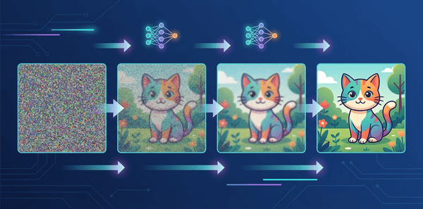
A diffusion model is trained to reverse a corruption process. Everything else follows from that. During training it watches images destroyed by noise in small increments and learns to undo each one, then at generation time runs that reversal on noise that was never an image.
The same mathematics drives motion as well as stills. An AI video generator applies the identical denoising framework across a sequence of frames rather than one, which is why platforms like ImagineArt run image and video models side by side. The statistics do not change, only the dimensionality.
The Forward Process
Take a training image and add a small amount of Gaussian noise. Repeat for several hundred to a thousand steps, each time adding noise to the already-noisy result. This is a Markov chain: each state depends only on the one before it, which makes the construction tractable.
After enough steps the original is unrecoverable and what remains is indistinguishable from pure noise. This process requires no learning at all. It follows a fixed variance schedule, where each step adds a predetermined amount of noise.
Why Gaussian Noise Specifically
The choice is not arbitrary.
- Gaussians are closed under addition, so a sum of normal variables is itself normal
- That gives a closed form for any step, so training can jump straight to step 400 without simulating the first 399
- When each step is small, the reverse of a Gaussian step is also approximately Gaussian, which is what makes the reversal learnable
- The distribution is specified by mean and variance alone, so there are only two quantities to estimate
That third point is load-bearing. If the forward steps were large, the reverse distribution would be complex and multimodal. Keeping them small is what guarantees the model only has to learn a Gaussian.
The Reverse Process
Now run it backwards. Start from pure noise and ask what this looked like one step earlier. The model estimates that, subtracts a little noise, and repeats until step zero. The output is an image that was never in the training set but comes from the same learned distribution.
What the Model Actually Predicts
Here is the part people get wrong. The network does not predict the clean image. In the standard formulation it predicts the noise that was added, and the cleaner estimate comes from subtracting that prediction.
Training is then a regression problem. Take an image, pick a random timestep, add the corresponding noise, and ask the network to recover it. The loss is mean squared error between true and predicted noise.
Guidance and the Diversity Trade-Off
Text prompts enter through conditioning. The model produces one noise estimate conditioned on your prompt and one unconditioned, then extrapolates away from the unconditioned one by a factor called the guidance scale.
- Low guidance gives varied output that may ignore parts of the prompt
- High guidance follows the prompt closely but collapses variety and can oversaturate
- The useful range is narrower than most interfaces suggest
That trade-off between fidelity and diversity is a variance problem, and it is why two people get very different results from the same words.
Where the Randomness Comes From
Every generation begins with a draw from a standard normal distribution, produced by a pseudorandom number generator, so it is reproducible.
Fix the seed, prompt, model, and sampler, and you get the same image every time. In a well-built AI image generator, locking the seed lets you change one prompt term and see only that change rather than an entirely new composition. ImagineArt exposes this across roughly forty models, which makes comparing engines from an identical starting point straightforward. Reproducibility is the difference between experimenting and guessing.
From Images to Video
Video adds a dimension rather than new theory. Instead of denoising one array of pixels, the model denoises a sequence while enforcing consistency across frames.
- Temporal attention lets each frame condition on its neighbours
- Noise is correlated across frames rather than drawn independently
- Clip length is bounded mostly by memory, which is why outputs cap near ten seconds
Conclusion
Diffusion models look like magic from outside and like a statistics problem from inside. A fixed Markov chain destroys training images with Gaussian noise, a network learns to estimate what was added at each step, and generation runs that estimation backwards from a fresh noise sample. The Gaussian choice is deliberate, the guidance scale is a variance trade-off, and the seed is the state of a pseudorandom generator. None of it requires taking anything on faith, which is the best argument for learning the underlying probability rather than treating these tools as black boxes.
Frequently Asked Questions
Why do diffusion models use so many steps?
Each reverse step is only approximately Gaussian, and that approximation holds when steps are small. More steps means better approximations. Modern samplers cut the count substantially by solving the underlying equation more efficiently.
Does the same seed always give the same image?
Yes, provided the prompt, model, sampler, and step count are also identical. The seed sets the initial noise draw, and the rest of the process is deterministic given that starting point.
Are diffusion models copying their training data?
Not in the ordinary sense. They learn a distribution and sample from it, so output is new. Memorisation can occur when an image is heavily duplicated in the training data, but that is the exception rather than the mechanism.
Diffusion models look like magic from outside and like a statistics problem from inside. The Gaussian choice is deliberate, the guidance scale is a variance trade-off, and the seed is the state of a pseudorandom generator.