
What Is the Law of Small Numbers?
The law of small numbers names a cognitive bias: expecting a small sample to mirror its population as closely as a large one would. Amos Tversky and Daniel Kahneman described it in "Belief in the Law of Small Numbers," a 1971 Psychological Bulletin paper. People, they wrote, treat a random sample as "highly representative, that is, similar to the population in all essential characteristics."
Its namesake, the law of large numbers, really is a theorem: very large samples do come to resemble their population. People's intuitions, the authors argued, behave as if that law "applies to small numbers as well." Training doesn't cure it: the authors' questionnaire went to professional psychologists, and their typical respondent was a believer.
The phrase can also mean a book by Ladislaus Bortkiewicz or the Poisson distribution; here it means the bias.
Why a Perfect Record on a Few Cases Proves So Little
Large samples settle near the true rate; small ones swing. Suppose a contractor really passes 90% of final inspections. The chance of a clean 3 out of 3 is 0.9 × 0.9 × 0.9 = 0.729, so nearly three times in four the record looks perfect.
Longer records leave luck less room. A clean 10 out of 10 still turns up 34.9% of the time, but a clean 100 out of 100 about once in 38,000 tries. So 100% on three jobs says little, and 95% on a hundred says a lot.
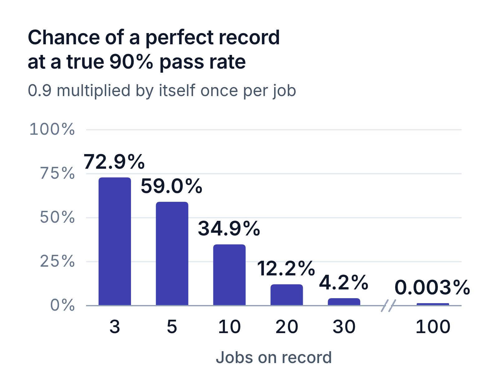
At a true 90% rate, a perfect record is likely on 3 jobs and almost impossible on 100: 72.9% on 3 jobs, 59.0% on 5, 34.9% on 10, 12.2% on 20, 4.2% on 30 and 0.003% on 100.
The same intuition feeds the gambler's fallacy, the hunch that a streak must soon reverse. Tversky and Kahneman's reply: deviations "are not canceled as sampling proceeds, they are merely diluted."
Where Rankings Fall for It (and How One Open Ranking Avoids It)
Every ranking built on shares must decide what a 3-out-of-3 record is worth. For local service firms on usd.org, the answer is written into the published formula of the permit check. It takes the share of a company's completed building permits that closed with a passing final inspection and scores it by a 90% Wilson interval's lower bound. Under 10 completed permits, the share isn't scored at all.
Here's why. Take 20 equally good contractors who each pass 90% of inspections, ten with 3 jobs and ten with 100. Sorted by raw share, on average about seven small firms tie for first at 100%, and the rest drop to 67% or lower, below all ten large firms.
The smallest records crowd both ends of such lists, from review scores to conversion tests. Researchers fall for it too: Tversky and Kahneman's believer bets on small samples and "overestimates power." A fair ranking needs a minimum count and a score that discounts thin evidence.
Rank With the Wilson Lower Bound, Not the Raw Share
The Wilson score interval, introduced in 1927, wraps an observed share in a range of plausible true rates. Its lower bound, the lowest rate your data still back at your chosen confidence, makes a cautious score that climbs toward the share as cases pile up.
The bound is one line of algebra in successes, cases and z (1.64 for 90% confidence, 1.96 for 95%). For a perfect record it shrinks to n ÷ (n + z²): 3 out of 3 at 90% gives 3 ÷ 5.69 = 0.53. The NIST/SEMATECH e-Handbook of Statistical Methods, which prints the full formula, notes that the method's worth "does not strongly depend upon the value of n and/or p" and that "the lower limit cannot be negative," unlike the most common formula.
| Record | Raw share | Wilson lower bound, 90% | Wilson lower bound, 95% |
|---|---|---|---|
| 3 of 3 | 100% | 0.53 | 0.44 |
| 9 of 10 | 90% | 0.65 | 0.60 |
| 10 of 10 | 100% | 0.79 | 0.72 |
| 19 of 20 | 95% | 0.80 | 0.76 |
| 30 of 30 | 100% | 0.92 | 0.89 |
| 95 of 100 | 95% | 0.90 | 0.89 |
| 950 of 1,000 | 95% | 0.94 | 0.93 |
Lower bounds calculated with the Wilson formula (z = 1.64 for 90%, 1.96 for 95%).
By raw share, 3 of 3 ties for first; by its lower bound it comes last, behind even 9 of 10, while 95 of 100 keeps 0.90.
Small firms aren't buried for good: a clean 30 of 30 scores 0.92 at 90% and passes 95 of 100, as does any clean record from 25 of 25 up. At 95%, the two almost tie at 0.89, so your confidence level controls how hard small numbers get cut.
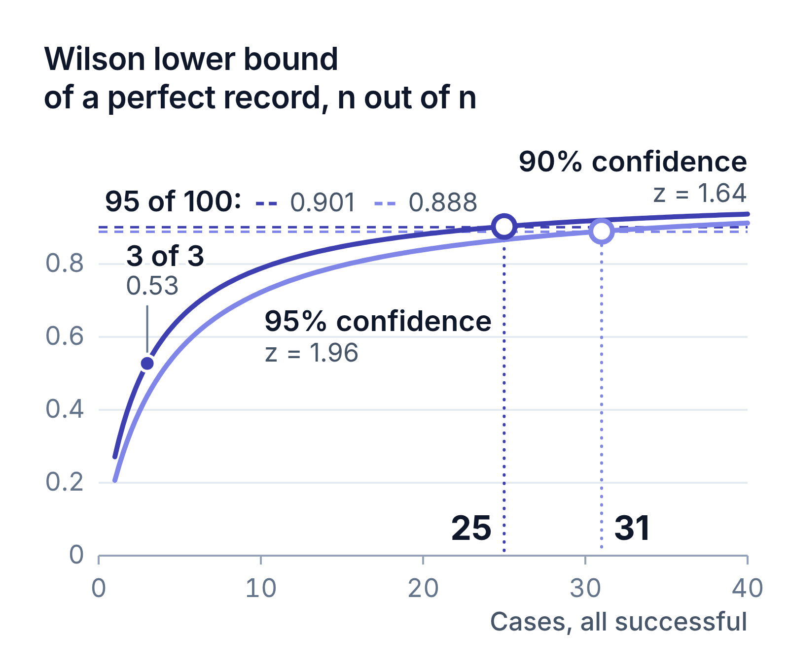
A clean record overtakes 95 of 100 at 25 cases (90%) and 31 cases (95%).
Three Rules That Keep a Small-Sample Ranking Honest
The permit check above adds three rules worth copying:
Rule 1 — Set a Minimum
- Set a minimum, and move the weight below it. Until a company has 10 completed permits, its share sits out and its weight shifts to permit volume.
- A zero would punish a firm for being new; a raw 100% would reward luck.
Rule 2 — Fix the Denominator
- Fix the denominator before you count. A final inspection counts only when its record says approved or passed.
- A permit that expired never counts as closed, so it weighs against the company, while a finished permit lacking any inspection record stays out of the share entirely.
Rule 3 — Let Volume Count
- Let volume count, with diminishing returns. Permit volume carries the remaining 50% of the check, with each extra permit worth less than the last until the count reaches the 75th percentile for its trade and city.
- Beyond it, more permits add nothing, so size alone can't carry the score.
Wilson Lower Bound or Bayesian Average?
A Bayesian average blends each record with a prior average, as if every company started with a few extra cases at that average. Take a prior of 85% worth 10 cases: 3 of 3 becomes (8.5 + 3) ÷ 13 = 0.88, and 95 of 100 becomes 0.94.
It also handles star scales, not only yes-or-no outcomes. But you pick the prior and its weight, and the weight matters: at the pull of a single case, 3 of 3 wins again, 0.96 to 0.95. The Wilson lower bound needs only the counts and a confidence level. Set up sensibly, either one keeps 3 out of 3 below 95 out of 100.
Frequently Asked Questions
What Is the Law of Small Numbers in Psychology?
It's an error of judgment, not a rule of statistics: Tversky and Kahneman traced it to a cognitive or perceptual bias. Believers overtrust small-sample conclusions and expect results to replicate more often than they do. Their remedy: "The obvious precaution is computation."
How Is the Law of Small Numbers Different From the Law of Large Numbers?
Only the second is a theorem: as a sample grows, its share settles near the true value. The first is a mistaken expectation that small samples behave the same way, so one describes how people misjudge chance and the other how chance behaves.
What Counts as a Small Sample?
There's no single cutoff. Near 100%, check the case count: at 90% confidence, 3 of 3 has a lower bound of 0.53 and 30 of 30 reaches 0.92. That's why a small sample size is bad for a ranking: it can't separate luck from skill. A 10-case minimum is a floor, not proof.
Key Takeaways
- A perfect short record is often luck: 72.9% of the time at a true 90% rate.
- Score shares with the Wilson lower bound: 3 of 3 falls to 0.53, 95 of 100 holds at 0.90.
- Below a minimum count, move the weight instead of scoring zero.
- Define success, failure and "neither" first, and cap what volume can earn.