Start With Visits and Converted Visits
Here, a converted visit means an eligible store visit with at least one purchase. Conversion is converted visits divided by eligible visits. These are visits, not unique customers or transaction counts; a real report needs a consistent counting rule across stores and periods.
| Store | Period | Visits | Converted Visits | Conversion |
|---|---|---|---|---|
| Oak Street | Before | 4,000 | 1,200 | 30% |
| Oak Street | After | 1,000 | 340 | 34% |
| Riverside | Before | 1,000 | 100 | 10% |
| Riverside | After | 4,000 | 480 | 12% |
Oak Street rises from 30% to 34%, an improvement of 4 percentage points. Riverside rises from 10% to 12%, an improvement of 2 points. Those increases describe rates, not purchase volume: Oak Street’s converted visits fall from 1,200 to 340 because its visit count falls sharply.
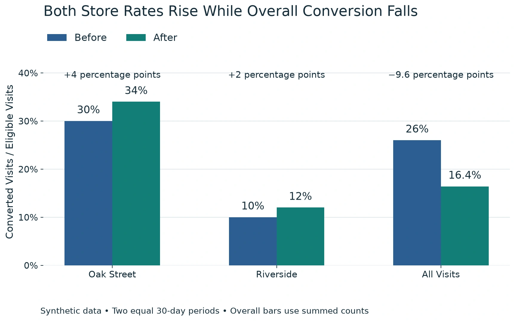
Across both stores, Before conversion is (1,200 + 100) / (4,000 + 1,000) = 26%. After conversion is (340 + 480) / (1,000 + 4,000) = 16.4%. Both periods have 5,000 visits, but converted visits fall from 1,300 to 820: 480 fewer, with a rate decline of 9.6 percentage points.
The store rates and company rate answer different questions. Neither finding should be discarded. Stanford’s explanation of Simpson’s paradox describes how a relationship within groups can reverse when the groups are combined. In this example, the counts show exactly how the reversal occurs; they do not establish what caused the traffic shift.
Explain the Changing Weights
The company rate is a visit-weighted mean of the two store rates. Oak Street represents 80% of visits Before and 20% After. Riverside’s share moves from 20% to 80%. These shares differ from each store’s conversion rate.
Before: (0.80 × 30%) + (0.20 × 10%) = 26%.
After: (0.20 × 34%) + (0.80 × 12%) = 16.4%.
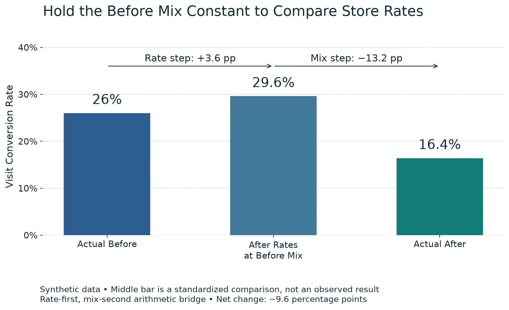
Riverside converts a smaller proportion of visits in both periods and now carries most of the weight. Its improvement cannot offset that redistribution. A plain average would rise from 20% to 23%, but it gives each store equal weight and therefore does not measure conversion across all visits. Statistics Fundmentals weighted-mean tutorial explains the distinction between a value and its weight.
Hold the Before Mix Constant
To compare the store rates without changing their weights, apply the Before visit shares to the After rates:
(0.80 × 34%) + (0.20 × 12%) = 29.6%.
At that fixed mix, conversion rises by 3.6 percentage points from the Before rate of 26%. The 29.6% result is a standardized comparison, not observed After conversion or a forecast.
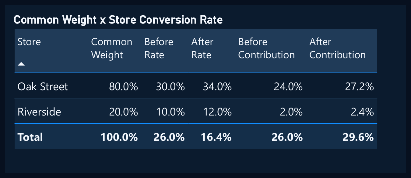
One arithmetic bridge moves from 26% to 29.6% using the new rates, then from 29.6% to 16.4% using the new visit mix. The rate step is +3.6 points; the mix step is −13.2 points; together they equal −9.6. This is a rate-first, mix-second decomposition. Reversing the order changes the allocation between steps, although the net change remains the same. Neither allocation proves causation.
Applied to 5,000 visits, the fixed-mix rate gives 1,480 converted-visit equivalents. The bridge is therefore +180 and −660, totaling −480. Those equivalents explain the arithmetic; the observed After count remains 820.
Reproduce the Result in Excel
The accompanying workbook contains the four-row Excel table, StorePeriod, and a Tutorial sheet. The source columns are Store, Period, Visits and ConvertedVisits. Each store-period pair must appear once, and converted visits must be between zero and visits. Proportional duplicate rows can leave a percentage looking correct while inflating its counts.
Use SUMIFS to collect the numerator and denominator separately. For Oak Street’s Before visits:
=SUMIFS(StorePeriod[Visits],StorePeriod[Store],"Oak Street",StorePeriod[Period],"Before")Repeat with StorePeriod[ConvertedVisits] for the numerator, then divide the two counts. Guard against a zero denominator; an undefined conversion rate is not 0%. Apply the same method to Riverside and After.
In the supplied Tutorial, B7:C8 hold Before counts and E7:F8 hold After counts. D7:D8 and G7:G8 calculate store rates. Row 9 sums counts before dividing: D9 is 26%, G9 is 16.4%, and H9 is −9.6 percentage points. A percentage-point difference multiplies the rate difference by 100 and uses a numeric format; percentage formatting would multiply it again.
Cells B16:B17 contain the Before weights, 80% and 20%. Multiply them by the After store rates and sum the contributions. F18 returns 29.6%, and F20 returns the +3.6-point fixed-mix change. Do not average the store percentages for the company total.
For a controlled check, change Oak Street’s After converted visits from 340 to 350. Its rate becomes 35%, actual company conversion becomes 16.6%, and the fixed-mix comparison becomes 30.4%. Restore 340 afterward. The workbook demonstrates two stores; adding more requires extending the cohort and calculation ranges rather than merely appending rows.
Reproduce the Result in Power BI
Import the supplied four-row CSV as StorePeriod. Set Store and Period to text and both count columns to whole numbers. Check uniqueness and count boundaries before creating measures.
Create a dedicated Metrics table using Enter Data, then add these measures there. Keeping them outside StorePeriod avoids confusing the Visits measure with its same-named source column.
Visits = SUM(StorePeriod[Visits])
Converted Visits = SUM(StorePeriod[ConvertedVisits])
Conversion Rate = DIVIDE([Converted Visits], [Visits])
DIVIDE returns blank for a zero denominator unless an alternative is specified. Leave that undefined result blank and format Conversion Rate as a percentage.
Create a separate Stores table with Oak Street and Riverside, then an active, single-direction, one-to-many relationship from Stores[Store] to StorePeriod[Store]. Use Stores[Store] for the slicer and matrix rows, Period for columns, and the three measures as values. Counts remain visible beside rates; totals divide summed counts.
In Power BI consulting, comparison cards need explicit periods while retaining the selected stores:
Before Rate =
    CALCULATE([Conversion Rate],
        REMOVEFILTERS(StorePeriod[Period]),
        StorePeriod[Period] = "Before")
After Rate =
    CALCULATE([Conversion Rate],
        REMOVEFILTERS(StorePeriod[Period]),
        StorePeriod[Period] = "After")
Conversion Change (pp) =
    VAR B = [Before Rate]
    VAR A = [After Rate]
    RETURN IF(NOT ISBLANK(B) && NOT ISBLANK(A),100*(A-B))
REMOVEFILTERS clears the named Period column here, not the store selection. Format the change as a number labeled in percentage points. The supplied complete measure file also contains denominator and cohort-coverage guards.
The fixed-mix measure needs a Before denominator and row counts. Define Before Visits by substituting [Visits] for [Conversion Rate] in Before Rate. Define Before Rows and After Rows similarly, using COUNTROWS(StorePeriod). Then add:
Standardized After Rate =
    VAR S = CALCULATETABLE(ALLSELECTED(Stores[Store]),
        REMOVEFILTERS(StorePeriod[Period]))
    VAR B = SUMX(S, [Before Visits])
    VAR MissingBefore = SUMX(S, IF([Before Rows] <> 1, 1, 0))
    VAR MissingAfter = SUMX(S, IF([Before Visits] > 0 &&
        ([After Rows] <> 1 || ISBLANK([After Rate])), 1, 0))
    RETURN IF(B > 0 && MissingBefore = 0 && MissingAfter = 0,
        DIVIDE(SUMX(S, VAR V = [Before Visits]
            RETURN IF(V = 0, 0, V * [After Rate])), B))
This sums Before weights multiplied by After rates. The independent Stores list retains a store with positive Before weight if its After row disappears. An absent or undefined After rate makes the comparison blank; it cannot silently remove that store.
The supplied report has Conversion Comparison and Traffic Mix And Standardization pages. The first compares observed counts and rates; the second exposes weights and weighted contributions.
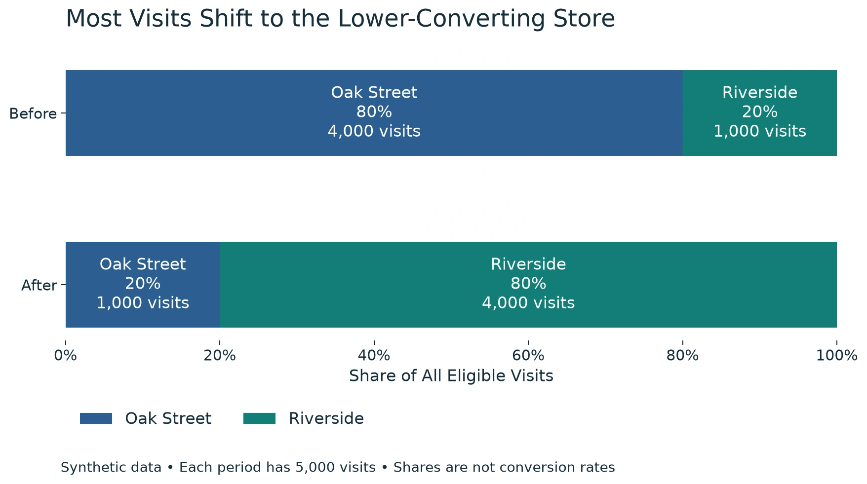
Test the saved report at All Stores, Oak Street and Riverside. Actual rates should be 26% → 16.4%, 30% → 34%, and 10% → 12%, respectively. The fixed-mix After results should be 29.6%, 34%, and 12%. A one-store selection has a 100% weight, so its standardized result equals its own After rate.
Decide What Needs Investigation
Start the data analytics review by verifying the counting rule, comparable trading windows and complete store coverage. Next inspect why the visit distribution changed. Campaigns, events or opening hours are possible questions for further records, not explanations proved by four rows. An improvement in conversion also says nothing by itself about basket value, merchandise cost or store profitability.
Data Pivot’s multi-store profitability example illustrates that separate financial question. Its transaction-to-visit ratio should not be confused with matched converted-visit measurement.
A practical goal of data visualization consulting is to present the headline rate, store rates and traffic weights together. Alder Lane’s example supports two simultaneous findings: both stores improved their conversion rates, and conversion across all visits fell. Showing the counts explains why; investigating operating records is what can explain the business cause.
Author Bio
Basem Fawzy is the founder of Data Pivot Consulting. He is a Microsoft Certified Power BI Developer and MBA graduate in E-Business with more than 10 years of experience in business intelligence, data modeling, dashboard development and reporting automation. He has worked with more than 200 clients and regularly translates operational data into management-level reporting frameworks.